- how to model the behavior of many assets simultaneously
- estimating correlation between asset price movements
- how to value and hedge options on many underlying assets in the Black-Scholes framework
- the pricing formula for European non-path-dependent options on dividend-paying assets
- how to price and hedge quantos and the role correlation
Multi-dimensional lognormal random walks
\[ dS_i = \mu_i S_i dt + \sigma_i S_i dX_i \]
\[ E[dX_i] = 0 ~ and ~ E[dX_i^2] = dt \]
but the random numbers \(dX_i\) and \(dX_j\) are correlated
\[ E[dX_i dX_j] = \rho_{ij}dt \]
correlation matrix
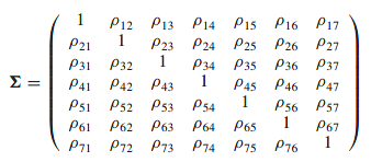
covariance matrix
\[ M \Sigma M \]
where M is the matrix with the \(\sigma_i\) along the diagonal and zeros everywhere else
Applying Ito’s lemma for multidimensional version
\[ dV = \left(\frac{\partial V}{\partial t} + \frac{1}{2}\sum_{i = 1}^d\sum_{j = 1}^d{\sigma_i \sigma_j \rho_{ij} S_i S_j \frac{\partial^2 V}{\partial S_i \partial S_j}} \right)dt + \sum_{i = 1}^d{\frac{\partial V}{\partial S_i}dS_i} \]
Using Taylor series and the rules of thumb
\[ dX_i^2 = dt ~ and ~ dX_idX_j = \rho_{ij}dt \]
Measuring correlations
return on the ith asset
\[ R_i(t_k) = \frac{S_i(t_k + \delta t) - S_i(t_k)}{S_i(t_k)} \]
historical volatility of the ith asset
\[ \sigma_i = \sqrt{\frac{1}{\delta t (M - 1)}\sum_{k = 1}^M{(R_i(t_k) - \bar{R_i})^2}} \]
where M is the number of data points in the return series and \(\bar{R_i}\) is the mean of all the returns in the series
the covariance is
\[ \frac{1}{\delta t (M - 1)}\sum_{k = 1}^M{(R_i (t_k) - \bar{R_i})(R_j(t_k) - \bar{R}_j)} \]
the correlation is
\[ \frac{1}{\delta t (M - 1)\sigma_i \sigma_j}\sum_{k = 1}^M{(R_i (t_k) - \bar{R_i})(R_j(t_k) - \bar{R}_j)} \]
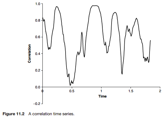
A historical correlation is not stable over the time series.
Implied correlation from the quoted price would be another instrument.
Options on many underlyings
Basket option, options on baskets, rainbow options
Portfolio consisting of 1 basket option and short a number \(\Delta_i\) of each of the asset
\[ \Pi = V(S_1, \dots, S_d, t) - \sum_{i = 1}^d{\Delta_i S_i} \]
\[ d\Pi = \left(\frac{\partial V}{\partial t} + \frac{1}{2}\sum_{i = 1}^d\sum_{j = 1}^d{\sigma_i \sigma_j \rho_{ij}S_i S_j \frac{\partial^2 V}{\partial S_i \partial S_j}} \right)dt + \sum_{i = 1}^d{(\frac{\partial V}{\partial S_i} - \Delta_i)}dS_i \]
\[ \Delta_i = \frac{\partial V}{\partial S_i} \]
\[ \frac{\partial V}{\partial t} + \frac{1}{2}\sum_{i = 1}^d\sum_{j = 1}^d{\sigma_i \sigma_j \rho_{ij}S_i S_j \frac{\partial^2 V}{\partial S_i \partial S_j}} + r\sum_{i = 1}^d{S_i \frac{\partial V}{\partial S_i}} - rV = 0 \]
Multidimensional version of the Black-Scholes equation
\[ \frac{\partial V}{\partial t} + \frac{1}{2}\sum_{i = 1}^d\sum_{j = 1}^d{\sigma_i \sigma_j \rho_{ij}S_i S_j \frac{\partial^2 V}{\partial S_i \partial S_j}} + \sum_{i = 1}^d{(r - D_i)S_i \frac{\partial V}{\partial S_i}} - rV = 0 \]
The pricing formula for European non-path-dependent options on dividend-paying assets

Exchanging one asset for another: a similarity solution
An exchange option gives the holder the right to exchange one asset for another, in some ratio.
The payoff for an exchange option at expiry
\[ \max{(q_1S_1 - q_2S_2, 0)} \]
\[ \frac{\partial V}{\partial t} + \frac{1}{2}\sum_{i = 1}^d\sum_{j = 1}^d{\sigma_i \sigma_j \rho_{ij}S_i S_j \frac{\partial^2 V}{\partial S_i \partial S_j}} + \sum_{i = 1}^d{(r - D_i)S_i \frac{\partial V}{\partial S_i}} - rV = 0 \]
\[ V(S_1, S_2, t) = q_1 S_2 H(\xi, t) \]
\[ \xi = \frac{S_1}{S_2} \]
\[ H(\xi, T) = max(\xi - \frac{q_2}{q_1}, 0) \]
the ratio q2/q1 plays the role of the strike

\[ \frac{\partial H}{\partial t} + \frac{1}{2}\sigma'^2\xi^2\frac{\partial^2 H}{\partial \xi^2} + (D_2 - D_1)\xi\frac{\partial H}{\partial \xi} - D_2H = 0 \]
\[ \sigma' = \sqrt{\sigma_1^2 - 2\rho_{12}\sigma_1 \sigma_2 + \sigma_2^2} \]
\[ V(S_1, S_2, t) = q_1 S_1 e^{-D_1(T - t)}N(d_1') - q_2S_2e^{-D_2(T - t)}N(d_2') \]
\[ d_1' = \frac{\log{(q_1 S_1 / q_2 S_2)} + (D_2 - D_1 + \frac{1}{2}\sigma r^2)(T - t)}{\sigma' \sqrt{T - t}} ~ and ~ d_2' = d_1' - \sigma'\sqrt{T - t} \]
\[ \frac{\partial V}{\partial S_1} = q_1 \frac{\partial H}{\partial \xi} \]
\[ \frac{\partial V}{\partial S_2} = q_1 H - q_1 \xi \frac{\partial H}{\partial \xi} \]
\[ \Pi = V - \Delta_1 S_1 - \Delta_2 S_2 \]
Quantos
Quanto is the cross-currency contract. The quanto has a payoff defined with respect to an asset or an index (or an interest rate) in one country, but then the payoff is converted to another currency for payment.
- ex) call on the Nikkei Dow index paid in US dollar
Define \(S_\$\) to be the yen-dollar exchange reate (number of dollars per yen) and \(S_N\) is the level of the Nikkei Dow index.
\[ dS_\$ = \mu_\$S_\$dt + \sigma_\$S_\$dX_\$ ~ and ~ dS_N = \mu_NS_Ndt + \sigma_NS_NdX_N \]
with a correlation coefficient \(\rho\) between them.
Hedged portfolio is
\[ \Pi = V(S_\$, S_N, t) - \Delta_\$S_\$ - \Delta_NS_NS_\$ \]
\(\Delta_\$\) is the number of yen short
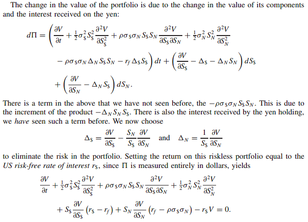
\[ V(S_\$, S_N, T) = max(S_N - E, 0) \]
\[ V(S_\$, S_N, t) = W(S_N, t) \]
\[ \frac{\partial W}{\partial t} + \frac{1}{2}\sigma_N^2 S_N^2\frac{\partial^2 W}{\partial S_N^2} + S_N \frac{\partial W}{\partial S_N}(r_f - \rho\sigma_\$\sigma_N) - r_\$V = 0 \]
The quanto is equivalent to using a dividend yield of
\[ r_\$ - r_f + \rho\sigma_\$\sigma_N \]
The only noticeable effect of the cross-currency feature on the option value is an adjustment to a dividend yield. This yield depends on the volatility of the exchange rate and the correlation between the underlying and the exchange rate.
Other features
Basket option
- early exercise
- path dependency
Sometimes the payoff is in one asset with a feature such as early exercise being dependent on another asset.
\[ \frac{\partial V}{\partial t} + \frac{1}{2}\sum_{i = 1}^2\sum_{j = 1}^2{\sigma_i \sigma_j \rho_{ij}S_i S_j\frac{\partial^2 V}{\partial S_i \partial S_j}} + \sum_{i = 1}^2{rS_i\frac{\partial V}{\partial S_i}} - rV = 0 \]
\[ V(S_1, S_2, T) = P(S_1) \]
\[ V(S_1, S_2, t) \geq P(S_1) ~ for ~ S_2 > E_2 \]
Realities of pricing basket options
The factors that determine the ease or difficulty of pricing and hedging multi-asset options are
- existence of a closed-form solution
- number of underlying assets, the dimensionality
- path dependency
- early exercise
The solution technique that we use will generally be one of
- finite-difference solution of a partial differential equation
- numerical integration
- Monte Carlo simulation
Easy problems
- closed-form solution
- no path-dependency
Medium problems
- low dimensionality
- early exercise
- many path-dependent features
Monte Carlo simulations are good for higher dimensions. It can cope with all path-dependent features, but not efficient for American-style early exercise.
Hard problems
- high dimensionality
- early exercise
- no numerical method
Realities of hedging basket options
The correlation is a very difficult quantity to measure. → Hedge ratios are very likely to be inaccurate.
To reduce sensitivity to parameters in delta hedging, vega hedging could be used.
Correlation versus cointegration
Because correlation is too unstable, cointegration could be an alternative statistical measure. Generally, the two series never stray too far from one another. This is probably a more robust measure of the linkage between two financial quantities.
Further reading
