The duration of a security with price P is the (negative of the ) percentage sensitivity of the price P to a small parallel shift in the level of interest rates. That is, let r(t, T) be the continuously compounded term structure of interest rates at time t. Consider a uniform shift of size dr across rates that brings rates to \(\bar r (t, T)\), given by
\[ r(t, T) \to \bar r (t, T) = r(t, T) + dr \]
\[ P \to \bar P = P + dP \]
\[ Duration = D_P = -\frac{1}{P}\frac{dP}{dr} \]
Given a duration \(D_P\) of a security with price P, a uniform change in the level of interest rates brings about a change in the value of
\[ \text{Change in portfolio value} = dP = - D_P \times P \times dr \]
Let A and a be two constants and x be a variable. Let \(F(x) = A \times e^{ax}\) be a function of x. Then, the first derivative of F with respect to x, denoted by dF/dx, is given by
\[ \text{Derivative of }F(x) \text{ with respect to }x = \frac{dF}{dx} = A \times a \times e^{ax} = a \times F(x) \]
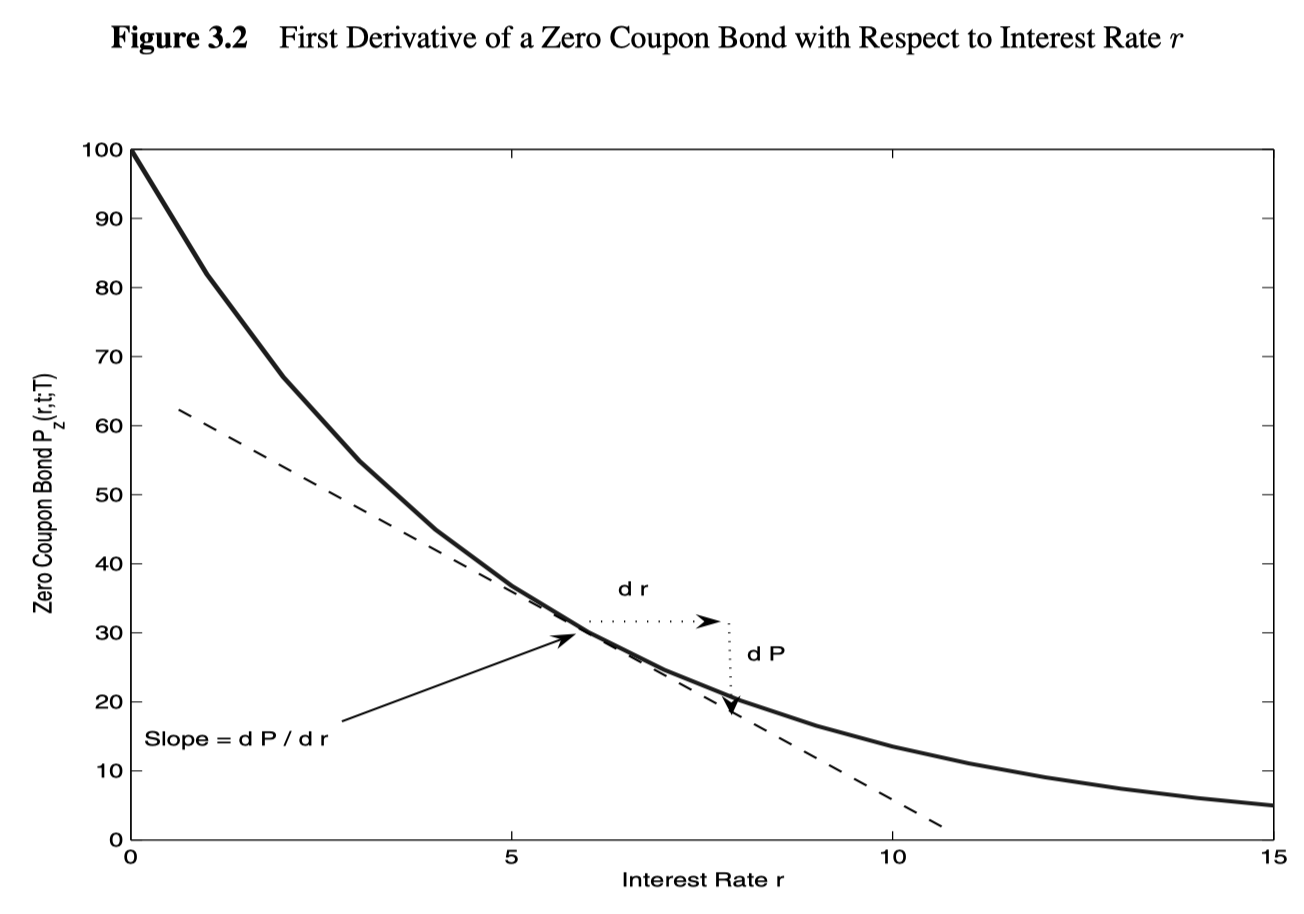
Lets \(P_z(r, t, T)\) be the price of a zero coupon bond at time t with maturity T and continuously compounded interest rate r. The first derivative of \(P_z(r, t, T)\) with respect to r is
\[ \frac{dP_z}{dr} = -(T - t) \times P_z(r, t, T) \]
Visually, the first derivative represents the slope of the curve \(P_z(r, t, T)\), plotted against r, at the current interest rate level.
Duration of a zero coupon bond
\[ D_{z, T} = -\frac{1}{P_z(r, t, T)}\frac{dP_z(r, t, T)}{dr} = T - t \]
Duration of a portfolio
\[ W = N_1 \times P_1 + N_2 \times P_2 \]
\[ \text{Duration of portfolio} = -\frac{1}{W}\frac{dW}{dr} = w_1 D_1 + w_2 D_2 \]
\[ w_1 = \frac{N_1 \times P_1}{W}, ~ w_2 = \frac{N_2 \times P_2}{W} \]
The duration of portfolio of n securities is given by
\[ D_W = \sum_{i = 1}^n{w_i D_i} \]
Duration of a coupon bond
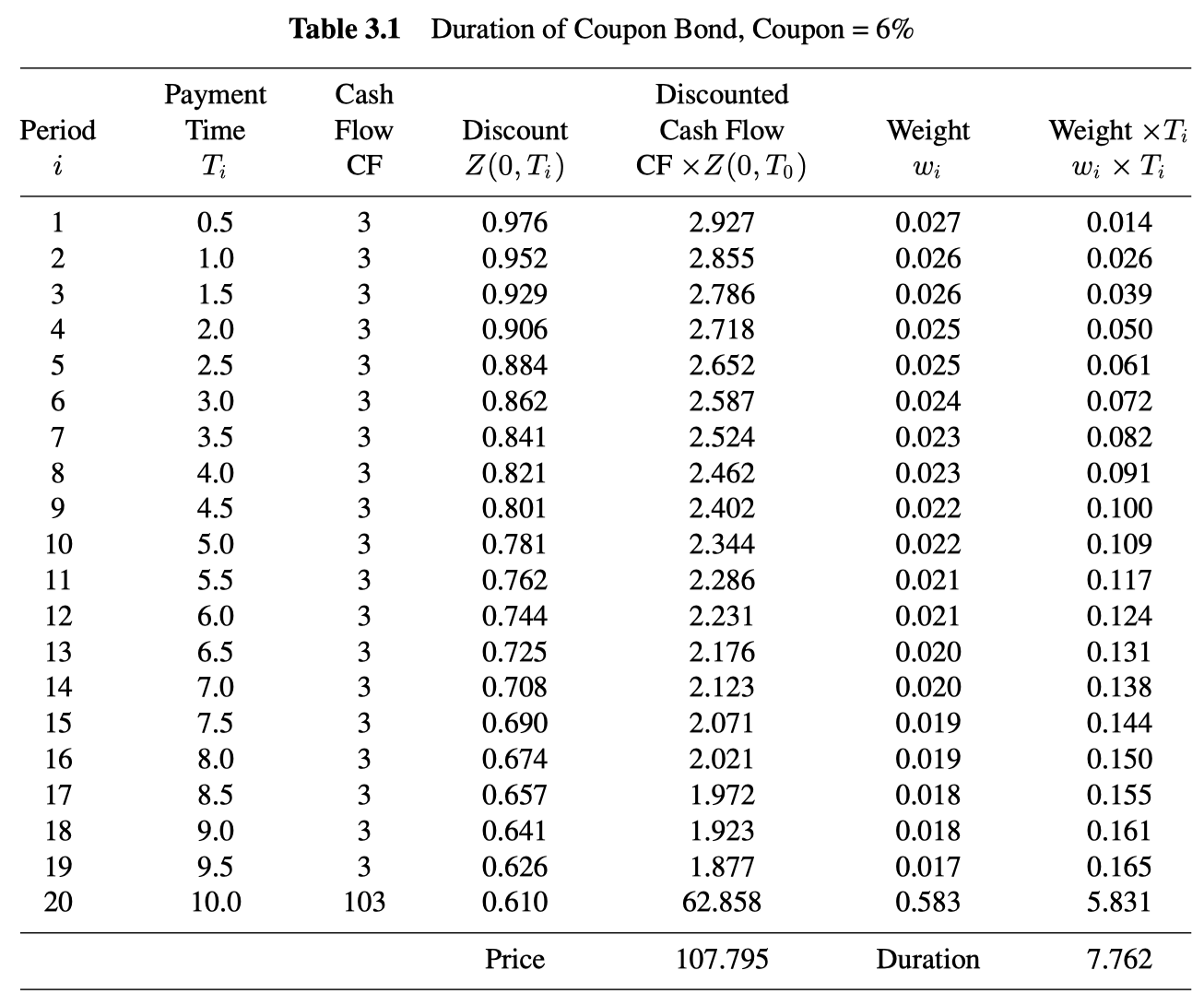
\[ P_c(0, T_n) = \sum_{i = 1}^{n - 1}{\frac{c}{2} \times P_z(0, T_i)} + (1 + \frac{c}{2})P_z(0, T_n) \]
\[ w_i = \frac{c/2 \times P_z(0, T_i)}{P_c(0, T_n)}~for~i = 1, \dots, n - 1 \]
\[ w_n = \frac{(1 + c/2) \times P_z(0, T_n)}{P_c(0, T_N)} \]
\[ D_c = \sum_{i = 1}^n{w_i T_i} \]
Duration and average time of cash flow payments
While we have derived the formula for duration from the definition of duration as the percentage sensitivity of a security to changes in interest rates, some confusion sometimes arises about the notion of duration because sometimes people define duration as the average time of payments. These two interpretations are equivalent for fixed rate bonds, that is, bonds that pay fixed coupons.
Properties of duration
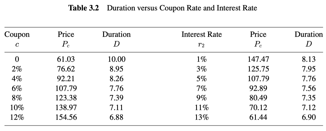
- lower average time of cash flow payments: the higher the coupon, the larger are the intermediate coupons relatively. Thus, the average time of coupon payments gets closer to today.
- lower sensitivity to interest rates: the higher the coupon rate, the larger are cash flows in the near future compared to the long-term future. Cash flows that arrive sooner rather than later are less sensitive to changes in interest rates. Thus, an increase in coupon rate implies an overall lower sensitivity to changes in discount rates.
Traditional definitions of duration
The duration is not defined against the continuously compounded interest rate but rather against the semi-annually compounded yield to maturity. In this case, the definition of the modified duration as the (negative of the) sensitivity of prices to changes in interest rates does not correspond exactly to the simple formulas derived earlier, and a small adjustment is needed.
\[ P_c(0, T) = \sum_{j = 1}^n{\frac{c/2 \times 100}{(1 + \frac{y}{2})^{2 \times T_j}}} + \frac{100}{(1 + \frac{y}{2})^{2 \times T_n}} \]
\[ MD = -\frac{1}{P}\frac{dP}{dy} = \frac{1}{1 + \frac{y}{2}}\sum_{j = 1}^n{w_j \times T_j} \]
\[ w_j = \frac{1}{P_c(0, T)}\left(\frac{c/2 \times 100}{(1 + \frac{y}{2})^{2 \times T_j}}\right), ~ w_n = \frac{1}{P_c(0, T)}\left(\frac{100 \times (c / 2 + 1)}{(1 + \frac{y}{2})^{2 \times T_n}}\right) \]
Macaulay duration - the weighted average of cash flow maturities
\[ D^{MC} = \sum_{j = 1}^n{w_j \times T_j} \]
The duration of zero investment portfolio: dollar duration
\[ \text{dollar duation} = D_P^\$ = -\frac{dP}{dr} \]
For z non-zero valued security or portfolio with price P, the relation between duration and dollar duration is
\[ D_P^\$ = P \times D_P \]
The dollar duration of portfolio of n securities
\[ D_W^\$ = \sum_{i = 1}^n{N_i D_i^\$} \]
The price of a basis point of a security with price P is defined
\[ \text{price value of a basis point} = PV01(or~PVBP) = -D_P^\$ \times dr \]
Duration and value-at-risk
Value-at-Risk (VaR) is a risk measure that attempts to quantify the amount of risk in a portfolio. In brief, VaR answers the following question: with 95% probability, what is the maximum portfolio loss that we can expect within a given horizon, such as a day, a week or a month?
Let \(\alpha\) be a percentile and T a given horizon. The (100 - \(\alpha\))% T VaR of a portfolio P is the maximum loss the portfolio can suffer over the horizon T with \(\alpha\)% probability. In formulas, let \(L_T = -(P_T - P_0)\) denote the loss of a portfolio. over the horizon T (a profit if negative). The VaR is that number such that:
\[ Prob(L_T > VaR) = \alpha \% \]
Through duration, we can estimate the sensitivity of a portfolio of fluctuations in the interest rate.
\[ dP = - D_P \times P \times dr \]
Let dr have a normal distribution with mean \(\mu\) and standard deviation \(\sigma\). dP has a normal distribution with mean and standard deviation given by:
\[ \mu_P = - D_P \times P \times \mu ~ and ~ \sigma_P = D_P \times P \times \sigma \]
\[ dr \sim N(\mu, \sigma^2) \to dP \sim N(\mu_P, \sigma_P^2) \]
\[ 95\% ~VaR = -(\mu_P - 1.645 \times \sigma_P) \]
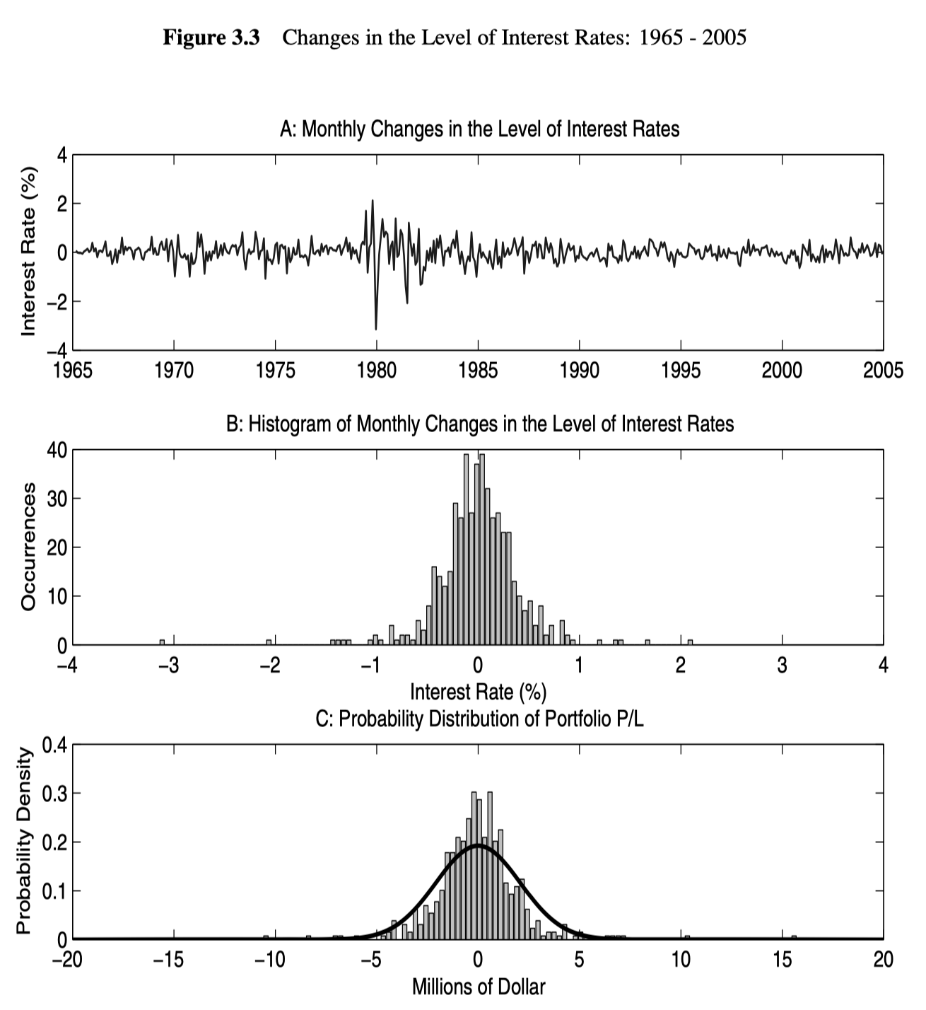
Warnings
- VaR is a statistical measure of risk, and as with any other statistical measure, it depends on distributional assumptions and the sample used for the calculation. The difference can be large.
- The duration approximation is appropriate for small parallel changes in the level of interest rates. However, by definition, VaR is concerned with large changes. Therefore, the duration approximation method is internally inconsistent.
- The VaR measures the maximum loss with 95% probability. However, it does not say anything about how large the losses could be if they do occur.
- The VaR formula includes the expected change in the portfolio \(\mu_P = - D_P \times P \times E[dr]\). The computation on the expected change E[dr] is typically very imprecise, and standard errors are large. Such errors can generate a large error in the VaR computation.
Duration and expected shortfall
Expected shortfall - This measure of risk answers the following question: how large can we expect the loss of a portfolio to be when it is higher than VaR?
The expected shortfall is the expected loss on a portfolio P over the horizon T conditional on the loss being larger than the (100 - \(\alpha\))%, T VaR:
\[ \text{Expected shortfall} = E[L_T | L_T > VaR] \]
\[ \text{95\% expected shortfall} = -(\mu_P - \sigma_P \times 2.0628) \]
The expected shortfall contains the same information as the VaR, as the only difference is the coefficient that multiplies \(\sigma_P\)