Quantitative Finance - Chapter 3 - the random behavior of assets

Untitled.png

In this chapter

• Jensen’s inequality
• how to examine time-series data to model returns
• the Wiener process, a mathematical model of randomness
• a simple model for equities, currencies, commodities and indices

The popular forms of ‘analysis’

Three form of ‘analysis’ commonly used in the financial world:

• Fundamental
• Technical
• Quantitative

Fundamental analysis is all about trying to determine the ‘correct’ worth of a company by an in-depth study of balance sheets, management teams, patent applications, competitors, lawsuit, etc.

Two difficulties

• very very hard
• Even if you have the perfect model for the value of a firm, it doesn’t mean you can make money.

Technical analysis is when you don’t care anything about the company other than the information contained within its stock price history.

Quantitative analysis is all about treating financial quantities such as stock prices or interest rates as random, and then choosing the best models for the randomness.

• forming a solid foundation for portfolio theory, derivatives pricing, risk management

Why we need a model for randomness: Jensen’s inequality

$$E[f(S)]\ge f(E[S])$$

where $\overline{S}=E[S]$, so that $E[ϵ]=0$. Then

$$E[f(S)]=E[f(\overline{S}+ϵ)]=E[f(\overline{S})+ϵf^{\prime }(\overline{S})+\frac{1}{2}{f}^{″}(S)+\dots ]\approx f(\overline{S})+\frac{1}{2}{f}^{″}(\overline{S})E[{ϵ}^2]=f(E[S])+\frac{1}{2}{f}^{″}(E[S])E[{ϵ}^2]$$

• $f^{″}(E[S])$: The convexity of an option. As a rule this adds value to an option. It also means that any intuition we may get from linear contracts (forwards and futures) might not be helpful with non-linear instruments such as options.
• $E[{ϵ}^2]$: Randomness in the underlying, and its variance. As stated above, modeling randomness is the key to modeling options.

Similarities between equities, currencies, commodities and indices

$$Return=\frac{\text{change in value of the asset}+\text{accumulated cashflows}}{\text{original value of the asset}}$$

Examining returns

The mean of the returns distribution is

$$\overline{R}=\frac{1}{M}\sum _{i=1}^M{R}_i$$

and the sample standard deviation is

$$\sqrt{\frac{1}{M-1}\sum _{i=1}^M(R_i-\overline{R}{)}^2)}$$

Supposing that we believe that the empirical returns are close enough to normal for this to be a good approximation.

$$R_i=\frac{S_{i+1}-S_i}{S_i}=mean+\text{standard deviation}\times \varphi$$

Timescales

Untitled

Call the time step $\delta t$. This mean of the return scales with the size of the time step. That is, the larger the time between sampling the more the asset will have moved in the meantime, on average.

$$mean=\mu \delta t$$

$$S_M=S_0(1+\mu \delta t{)}^M$$

$$S_M=S_0(1+\mu \delta t{)}^M=S_0{e}^{M\log (1+\mu \delta t)}\approx S_0{e}^{\mu M\delta t}=S_0{e}^{\mu T}$$

• In the absence of any randomness the asset exhibits exponential growth, just like cash in the bank.
• The model is meaningful in the limit as the time step tends to zero. If I had chosen to scale the mean of the returns distribution with any other power of $\delta t$ it would have resulted in either a trivial model ($S_T=S_0$) or infinite values for the asset ($S_T=\pm \mathrm{\infty }$).

$$\text{standard deviation}=\sigma \delta t^{1/2}$$

where $\sigma$ is some parameter measuring the amount of randomness; the larger this parameter the more uncertain is the return.

Putting these scaling explicitly into out asset return model

$$R_i=\mu \delta t+\sigma \varphi \delta t^{1/2}$$

$$S_{i+1}-S_i=\mu S_i\delta t+\sigma S_i\varphi \delta t^{1/2}$$

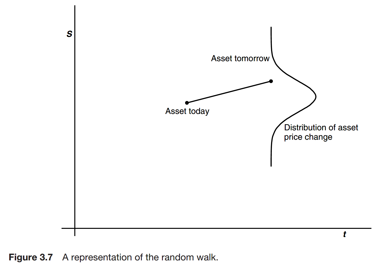
This equation as a model for a random work of the asset price.

The parameter $\mu$ is called the drift rate, the expected return or the growth rate of the asset. $\mu$ is quoted as an annualized growth rate.

$$\mu =\frac{1}{M\delta t}\sum _{i=1}^M{R}_i$$

The volatility

The parameter $\sigma$ is called the volatility of the asset. It can be estimated by

$$\sqrt{\frac{1}{(M-1)\delta t}\sum _{i=1}^M(R_i-\overline{R}{)}^2}$$

The volatility is the most important and elusive quantity in the theory of derivatives.

Because of their scaling with time, the drift and volatility have different effects on the asset path. The drift is not apparent over short timescales for which the volatility dominates. Over long timescales, for instance decades, the drift becomes important.

Estimating volatility

If $\delta t$ is sufficiently small the mean return $\overline{R}$ term can be ignored. For small $\delta t$

$$\sqrt{\frac{1}{(M-1)\delta t}\sum _{i=1}^M(\log S(t_i)-\log S(t_{i-1}){)}^2}$$

can also be used, where $S(t_i)$ is the closing price on day $t_i$

It is highly unlikely that volatility is constant in time. If you want to know the volatility today you must use some past data in the calculation. Unfortunately, this means that there is no guarantee that you are actually calculating today’s volatility.

Since all returns are equally weighted, while they are in the estimate of volatility, any large return will stay in the estimate of volatility until the 10 (or 30 or 100) days have passed. This gives rise to a plateauing of volatility, and is totally spurious.

Since volatility is not directly observable, and because of the plateauing effect in the simple measure of volatility, you might want to use other volatility estimates.

The random walk on a spreadsheet

$$S_{i+1}=S_i(1+\mu \delta t+\sigma \varphi \delta t^{1/2})$$

The Winer process

You can think of dX as being a random variable, drawn from a normal distribution with mean zero and variance dt:

Using Wiener process instead of normal distributions and discrete time, the important point is that we can build up a continuous-time theory.

The widely accepted model for equities, currencies, commodities and indices

$$dS=\mu Sdt+\sigma SdX$$

Stochastic differential equation is a continuous-time model for an asset price. It is the most widely accepted model.

Further reading

Untitled