In this chapter
- all the stochastic calculus
- the meaning of Markov and martingale
- Brownian motion
- stochastic integration
- stochastic differential equations
- Ito’s lemma in one and more dimensions
The Markov property
The distribution of the value of the random variable \(S_i\) conditional upon all of the past events only depends on the previous value \(S_{i - 1}\). This is the Markov property.
The martingale property
\[ E[S_i | S_j, j < i] = S_j \]
Quadratic variation
Quadratic variation of the random work
\[ \sum_{j = 1}^i{(S_j - S_{j - 1})^2} \]
Brownian motion
We will have n tosses in the allowed time t, with an amount \(\sqrt{t/n}\) riding on each throw. Again, the Markov and martingale properties are retained and the quadratic variation is still
\[ \sum_{j = 1}^i{(S_j - S_{j - 1})^2} = n \times (\sqrt{\frac{t}{n}})^2 = t \]
As I go to the limit \(n = \infty\), the resulting random walk stays finite. It has an expectation, conditional on a starting value of zero and a variance are
\[ E[S(t)] = 0,~E[S(t)^2] = t \]
I use S(t) to denote the amount you have won or the value of the random variable after a time t. The limiting process for this random walk as the time steps go to zero is called Brownian motion, and I will denote it by X(t).
- finiteness: Any other scaling of the bet size or ‘increments’ with time step would have resulted in either a random walk going to infinity in a finite time, or a limit in which there was no motion at all. It is important that the increment scales with the square root of the time step.
- Continuity: The paths are continuous, there are no discontinuous. Brownian motion is the continuous-time limit of our discrete time random walk.
- Markov: The conditional distribution of X(t) given information up until \(\tau < t\) depends only on \(X(\tau)\)
- Martingale: Given information up until \(\tau < t\) the conditional expectation of X(t) is \(X(\tau)\)
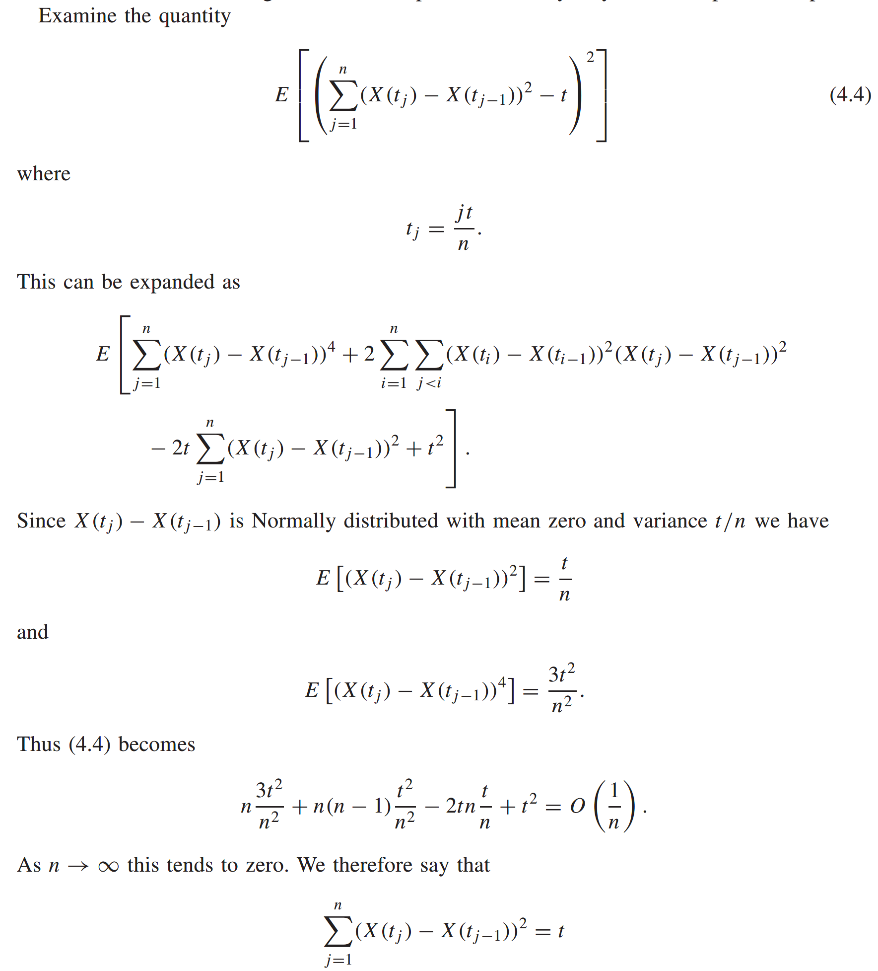
- Quadratic variation: If we divide up the time 0 to t in a partition with n + 1 partition points \(t_i = i t/n\) then
\[ \sum_{j = 1}^n{(X(t_j) - X(t_{j - 1}))^2} \to t \]
- Normality: Over finite time increments \(t_{i - 1}\) to \(t_i\), \(X(t_i) - X(t_{i - 1})\) is normally distributed with mean zero and variance \(t_i - t_{i - 1}\)
Stochastic integration
\[ W(t) = \int_0^t{f(\tau)dX(\tau)} = \lim_{n \to \infty}{\sum_{j = 1}^n{f(t_{j - 1})(X(t_j) - X(t_{j - 1}))}} \]
\[ t_j = \frac{jt}{n} \]
The integration is non-anticipatory.
Stochastic differential equations
\[ W(t) = \int_0^t{f(\tau)dX(\tau)} \]
\[ dW = f(t) dX \]
Think of dX as being an increment in X, i.e. a normal random variable with mean zero and standard deviation \(dt^{1/2}\)
\[ dW = g(t)dt + f(t)dX \]
\[ W(t) = \int_0^t{g(\tau)d\tau} + \int_0^t{f(\tau)dX(\tau)} \]
stochastic differential equations

Deterministic being a function representing the growth in something when you switch randomness off, and Random being another function representing how random the Something is.
The mean square limit
Functions of stochastic variables and Ito’s lemma
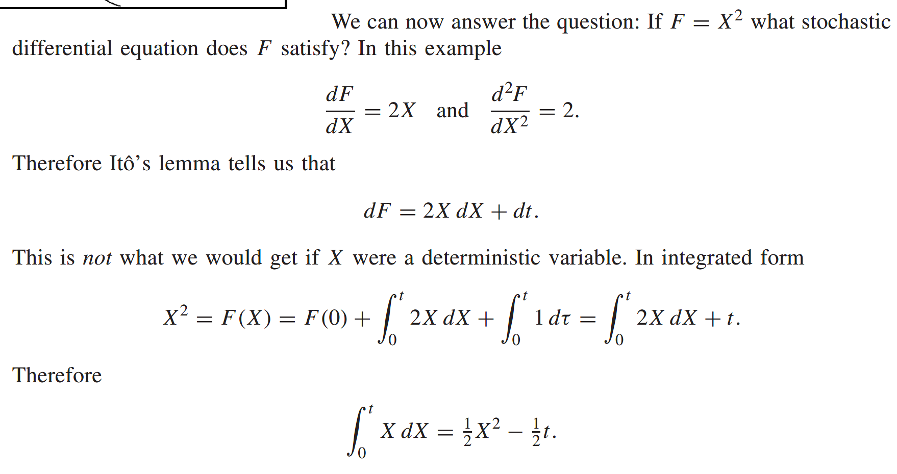
Clearly X is random and therefore F(X) is random, stochastic. If F is stochastic then what is the stochastic differential equation is satisfies?
If \(F = X^2\) is true that \(dF = eXdX\)?
No. The ordinary rules of calculus do not generally hold in a stochastic environment. Then what are the rules of calculus?
I am going to ‘derive’ the most important rule of stochastic calculus, Ito’s lemma.
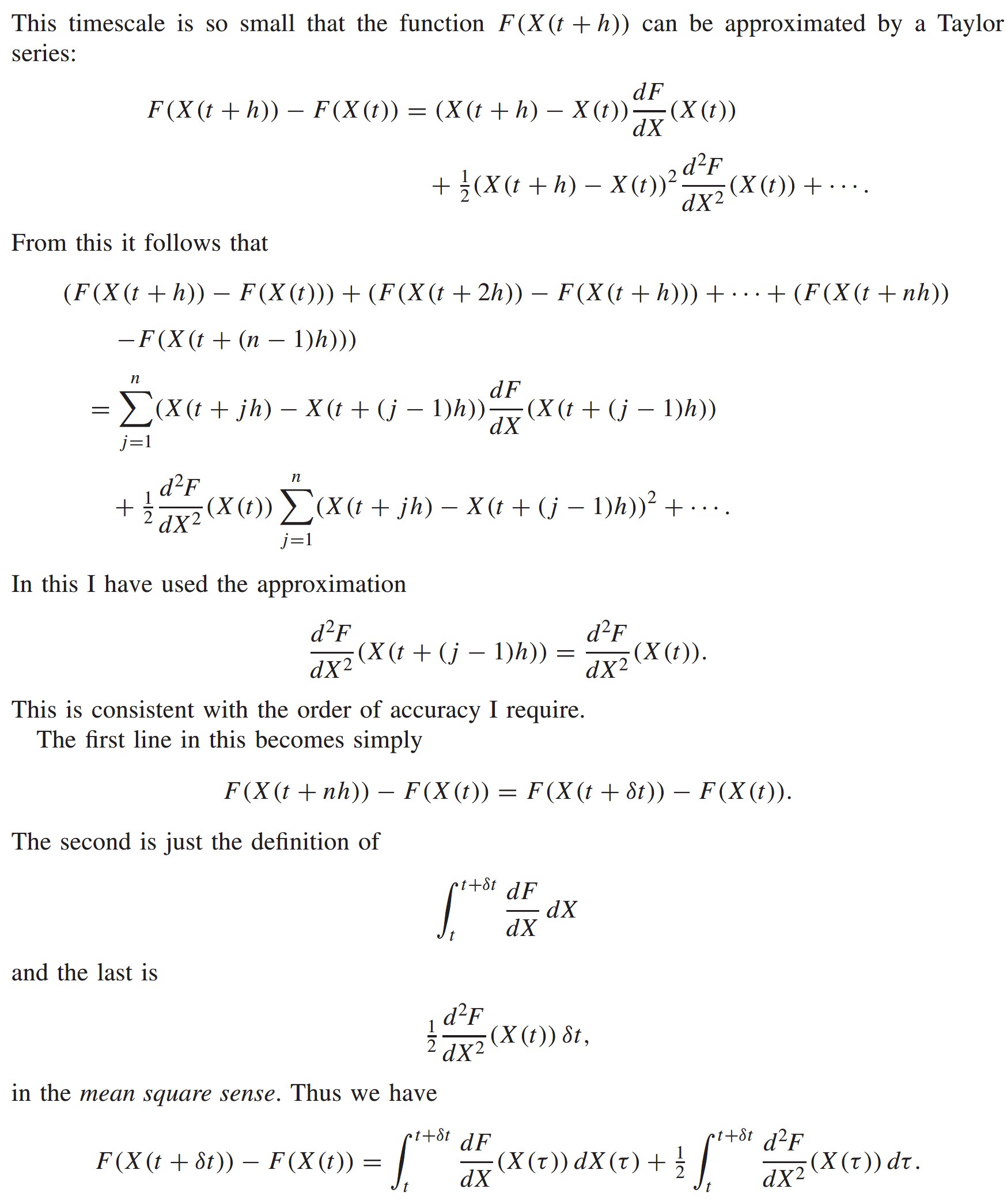
I can now extend this result over longer timescales, from zero up to t, over which F does vary substantially to get
\[ F(X(t)) = F(X(0)) + \int_0^t{\frac{dF}{dX}(X(\tau))dX(\tau)} + \frac{1}{2} \int_0^t{\frac{d^2F}{dX^2}(X(\tau))d\tau} \]
This is the integral version of Ito’s lemma.
\[ dF = \frac{dF}{dX}dX + \frac{1}{2}\frac{d^2F}{dX^2}dt \]
Interpretation of Ito’s Lemma
Both look stochastic and we know that the stock price satisfies a stochastic differential equation
\[ dS = \mu S dt + \sigma S dX \]
What are the underlined bits? And that is precisely what Ito tells us.
This will be important later when we do the Black-Scholes theory, because knowing how much randomness there is in an option’s value relative to a stock’s value will give us a recipe for eliminating the randomness by buying an option and selling short a special quantity of the stock.
Ito and Taylor
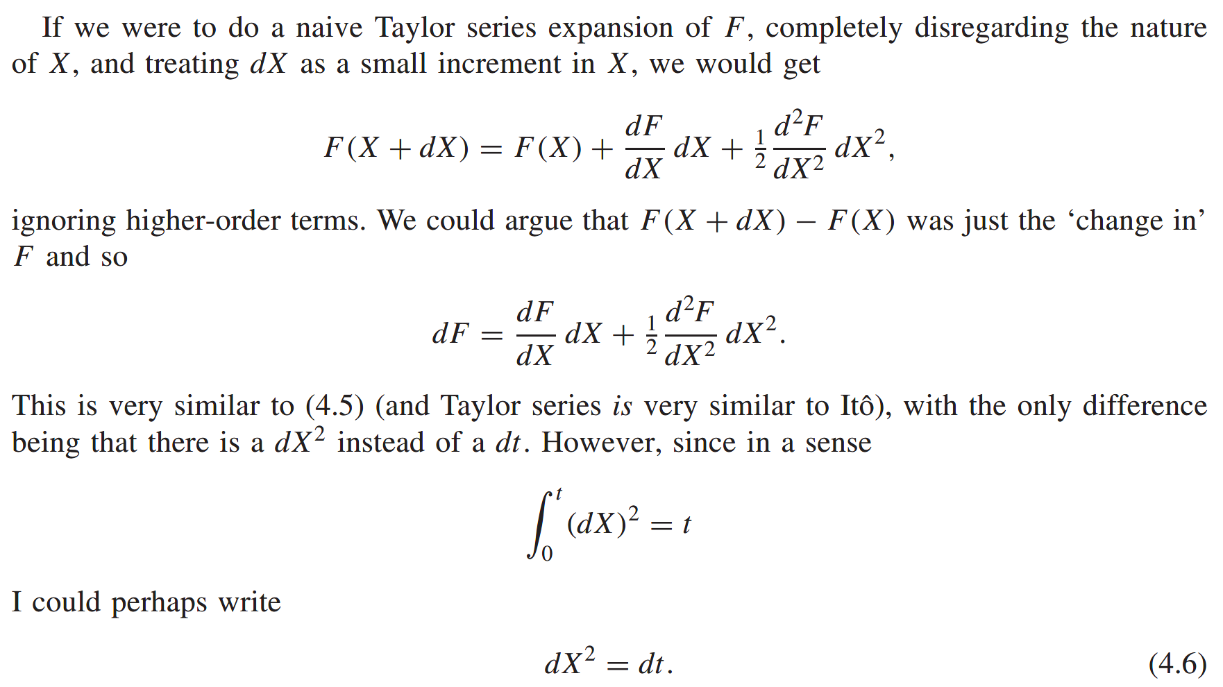
use Taylor series with the ‘rule of thumb’
The intuition
There are several contributions to the sum: Those that are a sum of random variables and those that are the sum of the squares of random variables, and then there are higher-order terms.
Add up a large number of random variables and the Central limit theorem kicks in, the end result being a normally distributed random variable. But what is its mean and standard deviation? This is the key.
The higher-order terms have means and standard deviations that are too small, disappearing rapidly in the limit as N tends to infinity.
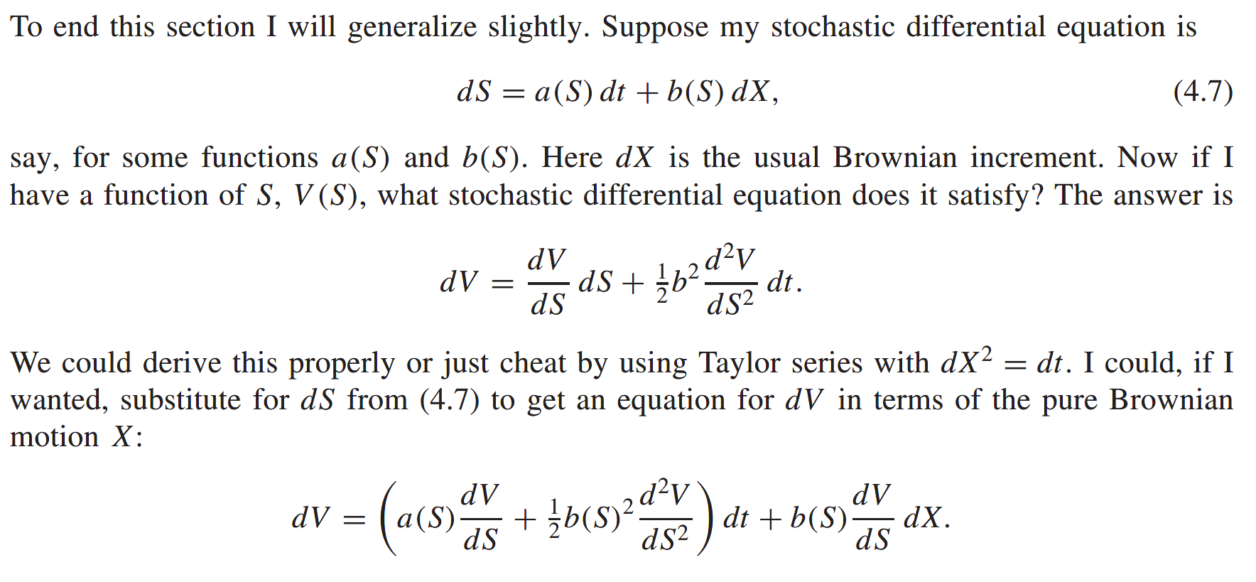
Simple generalization
spot price
- 1st derivative: return
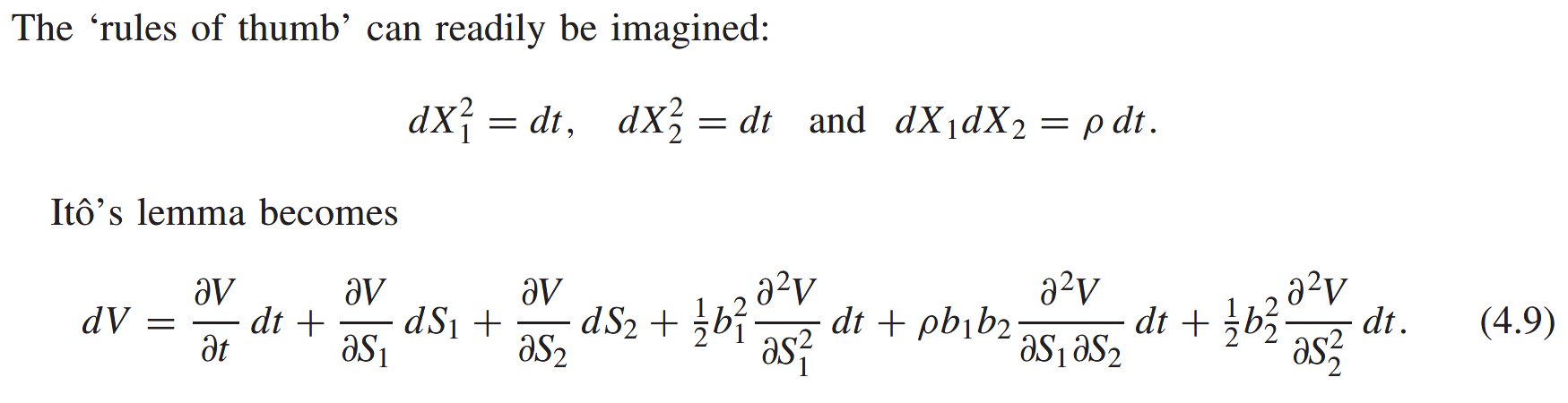
Ito in higher dimensions
They are correlated
Some pertinent examples
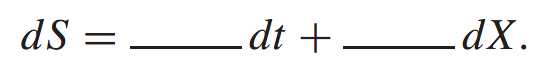
The bit in front of the dt is deterministic and the bit in front of the dX tells us how much randomness there is. Modeling is very much about choosing functions to go where the underlining is; it is about choosing the functional form for the deterministic part and the functional form for the amount of randomness.
Brownian motion with drift
\[ dS = \mu dt + \sigma dX \]
\[ S(t) = S(0) + \mu t + \sigma(X(t) - X(0)) \]
The lognormal random walk
\[ dS = \mu S dt + \sigma S dX \]
\[ dF = \frac{dF}{dS}dS + \frac{1}{2} \sigma^2 \S^2 \frac{d^2F}{dS^2}dt = \frac{1}{S}(\mu S dt + \sigma S dX) - \frac{1}{2} \sigma^2 dt = (\mu - \frac{1}{2}\sigma^2) dt + \sigma dX \]
\[ dV = \frac{\partial V}{\partial t} dt + \frac{\partial V}{\partial S} dS + \frac{1}{2} \sigma^2 S^2 \frac{\partial^2 V}{\partial S^2} dt \]
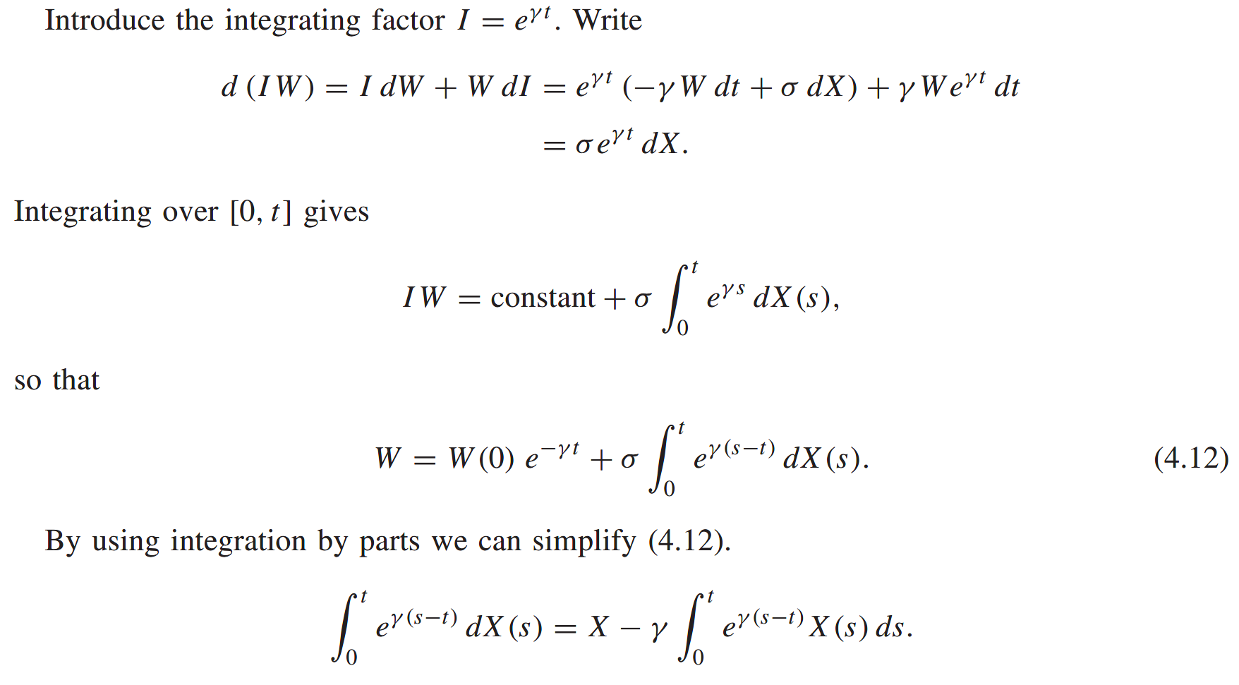
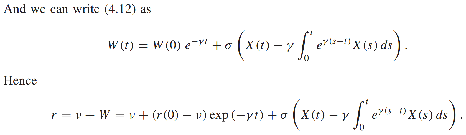
A mean-reverting random walk
\[ dS = (\nu - \mu S)dt + \sigma dX \]
This random walk is an example of a mean-revering random walk. If S is large, greater than \(\nu / \mu\), the negative coefficient in front of dt means that S will move down on average; if S is small, less than \(\nu / \mu\), it rises on average. There is still no incentive for S to stay positive in this random walk. With r instead of S this random walk is the Vasicek model for the short-term interest rate.
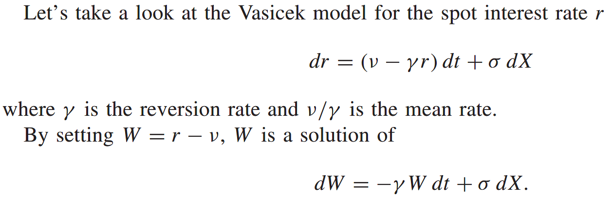
The random walk for W is an Ornstein-Uhlenbeck process.
And another mean-reverting random walk
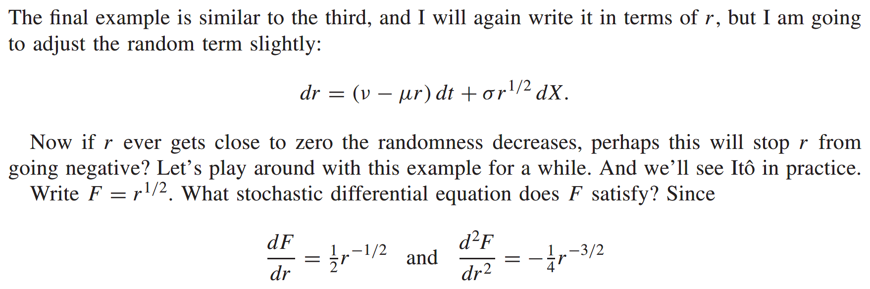
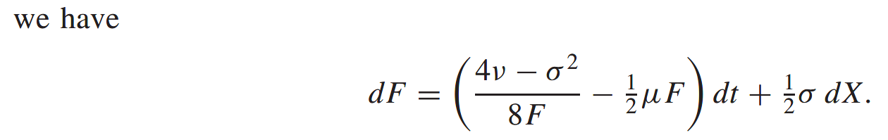
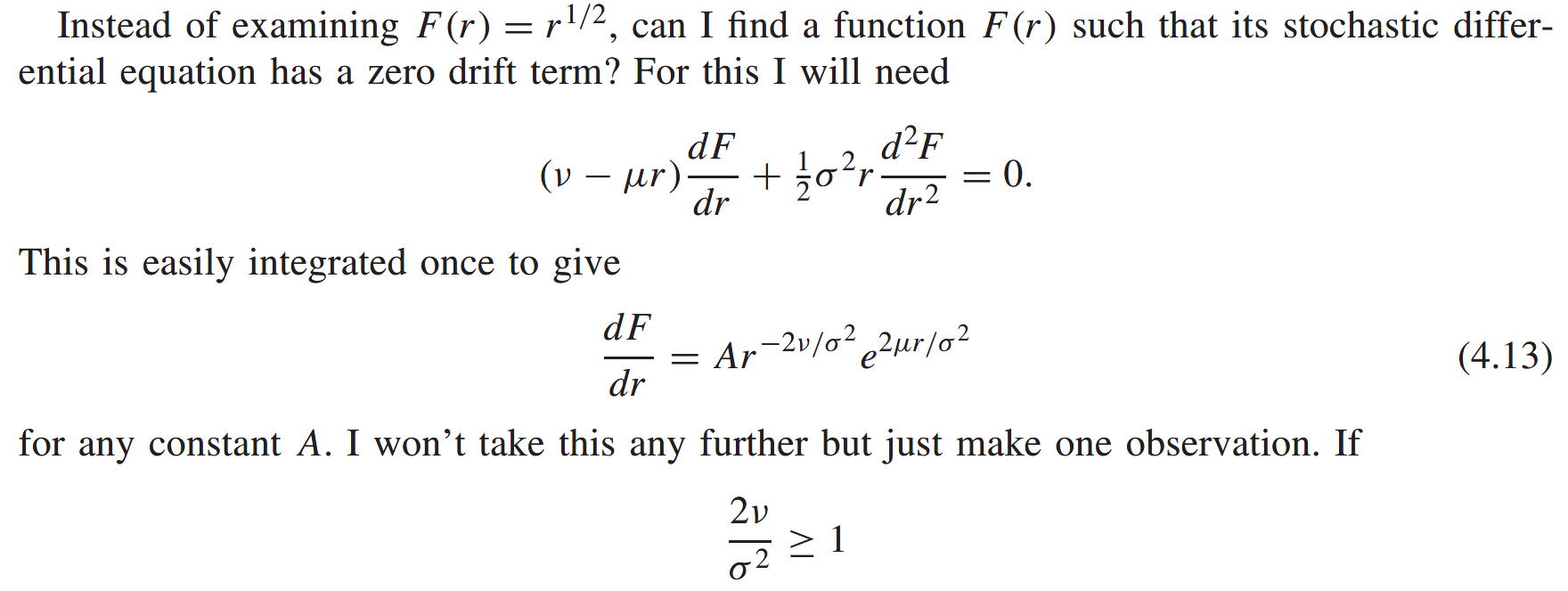
This makes the origin non-attainable. In other word, if the parameter \(\nu\) is sufficiently large it forces the random walk to stay away from zero.
Further reading