Quantitative Finance - Chapter 8 - simple generalizations of the Black-Scholes world

Untitled.png

• complex dividend structures
• jump conditions
• time-dependent volatility, interest rate and dividend yield

Dividends, foreign interest and cost of carry

Assume continuous dividend

• good for stock index incorporating large number of stocks
• underlying is currency taking foreign interest rate as a dividend yield

Dividend yield = cost of carry

$$\frac{\partial V}{\partial t}+\frac{1}{2}{\sigma }^2{S}^2\frac{{\partial }^{2}V}{\partial S^2}+(r-D)S\frac{\partial V}{\partial S}-rV=0$$

The reality is

• the amount of the dividend is not known until shortly before it is paid
• the payment is a given dollar amount, independent of the stock price
• the dividend is paid discretely

Dividend structures

Assume

• the amount of the dividend is known amount, possibly with some functional dependence on the asset value at the payment date
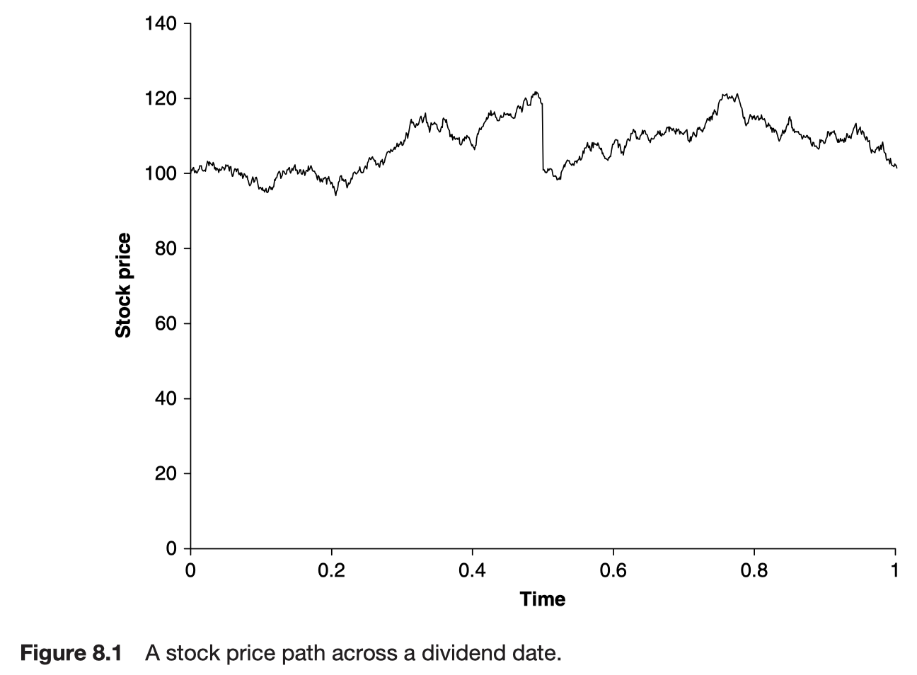
• the dividend is paid discretely on a known date

Dividend payments and no arbitrage

Untitled

$$S(t_i^{+})=S(t_i^{-})-D_i$$

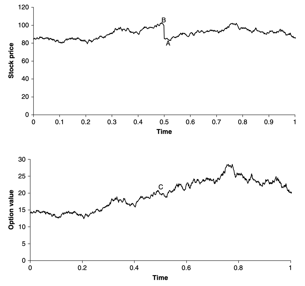
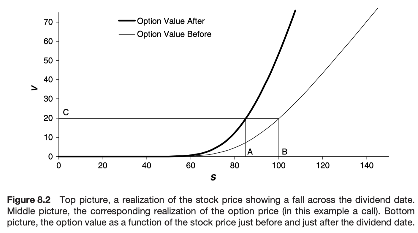
The behavior of an option value across a dividend date

jump condition

• discontinuous change in one of the independent variables

💡 How does this affect the option price?

Untitled

Untitled

$$V(S,t_i^{-})=V(S-D_i,t_i^{+})$$

Commodities

Convenience yield

• benefit associated with holding an underlying product or physical good

two types of commodity

• investment commodities - held for investment
• consumption commodities - held for consumption

Futures prices and arbitrage

consumption commodities

• Only an upper bound can be found because there may be constraints on the selling of consumption commodities

No arbitrage argument can still be applied to investment commodity futures.

Storage costs

No storage costs

$$F=S{e}^{r(T-t)}$$

Storage costs proportional to spot price, for investment commodities

$$F=S{e}^{(r+u)(T-t)}$$

Storage costs proportional to spot price, for consumption commodities

$$F\le S{e}^{(r+u)(T-t)}$$

This is because of commodities will be reluctant to sell the commodity which they are keeping for consumption.

• low price → do not sell
• high price → do not sell if they still need it

Convenience yield

$$F=S{e}^{(r+u-y)(T-t)}$$

with y ≥ 0.

For investment commodities y = 0.

Cost of carry

sum of storage cost, interest paid to finance the asset, less any income from the asset

The convenience yield is not included.

Effect on options

$$\frac{\partial V}{\partial t}+\frac{1}{2}{\sigma }^2{S}^2\frac{{\partial }^{2}V}{\partial S^2}+(r+u)S\frac{\partial V}{\partial S}-rV=0$$

$$F=S{e}^{(r+u-y)(T-t)}$$

$$H(F,t)=V(S,t)$$

$$\frac{\partial H}{\partial t}+\frac{1}{2}{\sigma }^2{F}^2\frac{{\partial }^{2}V}{\partial F^2}+yF\frac{\partial V}{\partial F}-rH=0$$

Stock borrowing and repo

To short stock, you have to borrow the stock from someone else by paying some interest for it.

lognormal random walk for the stock

$$dS=\mu Sdt+\sigma SdX$$

$$\mathrm{\Pi }=V(S,t)-\mathrm{\Delta }S$$

$$d\mathrm{\Pi }=dV-\mathrm{\Delta }dS$$

$$d\mathrm{\Pi }=\frac{\partial V}{\partial t}dt+\frac{\partial V}{\partial S}dS+\frac{1}{2}{\sigma }^2{S}^2\frac{{\partial }^{2}V}{\partial S^2}-\mathrm{\Delta }dS$$

incorporating interest expense

$$d\mathrm{\Pi }=\frac{\partial V}{\partial t}dt+\frac{\partial V}{\partial S}dS+\frac{1}{2}{\sigma }^2{S}^2\frac{{\partial }^{2}V}{\partial S^2}-\mathrm{\Delta }dS-Rmax(\mathrm{\Delta },0)Sdt$$

To eliminate the random terms

$$\mathrm{\Delta }=\frac{\partial V}{\partial S}$$

$$d\mathrm{\Pi }=(\frac{\partial V}{\partial t}dt+\frac{1}{2}{\sigma }^2{S}^2\frac{{\partial }^{2}V}{\partial S^2})-Rmax(\mathrm{\Delta },0)Sdt$$

This is deterministic portfolio to earn risk-free rate

$$d\mathrm{\Pi }=r\mathrm{\Pi }dt$$

$$\frac{\partial V}{\partial t}+\frac{1}{2}{\sigma }^2{S}^2\frac{{\partial }^{2}V}{\partial S^2}+rS\frac{\partial V}{\partial S}-rV-RSmax(\frac{\partial V}{\partial S},0)=0$$

Time-dependent parameters

When the interest rate, volatility and dividend yield/foreign interest rate are time dependent

$$\frac{\partial V}{\partial t}+\frac{1}{2}{\sigma }^2(t)S^2\frac{{\partial }^{2}V}{\partial S^2}+(r(t)-D(t))S\frac{\partial V}{\partial S}-r(t)V=0$$

$$\overline{S}=S{e}^{\alpha (t)}$$

$$\overline{V}=V{e}^{\beta (t)}$$

$$\overline{t}=\gamma (t)$$

To eliminate all time-dependent coefficient

$$\gamma (t)\frac{\partial \overline{V}}{\partial \overline{t}}+\frac{1}{2}\sigma (t{)}^2{\overline{S}}^2\frac{{\partial }^2\overline{V}}{\partial {\overline{S}}^2}+(r(t)-D(t)+\dot{\alpha }(t))\overline{S}\frac{\partial V}{\partial S}-(r(t)+\dot{\beta }(t))\overline{V}=0$$

$$\dot{}=d/dt$$

$$\beta (t)={\int }_t^{T}r(\tau )d\tau$$

$$\alpha (t)={\int }_t^T(r(\tau )-D(\tau ))d\tau$$

$$\gamma (t)={\int }_t^T{\sigma }^2(\tau )d\tau$$

$$\frac{\partial \overline{V}}{\partial \overline{t}}=\frac{1}{2}{\overline{S}}^2\frac{{\partial }^2\overline{V}}{\partial {\overline{S}}^2}$$

There is a coefficient which are independent of time.

$$V=e^{-\beta (t)}\overline{V}(S{e}^{\alpha (t)},\gamma (t))$$

$$r_c=\frac{1}{T-t}{\int }_t^{T}r(\tau )d\tau$$

$$D_c=\frac{1}{T-t}{\int }_t^{T}D(\tau )d\tau$$

$${\sigma }_c=\frac{1}{T-t}{\int }_t^T{\sigma }^2(\tau )d\tau$$

$$V_{BS}=e^{-r_c(T-t)}{\overline{V}}_{BS}(S{e}^{-(r_c-D_c)(T-t)},{\sigma }_c^2(T-t))$$

$$S{e}^{-{\int }_t^{T}D(\tau )d\tau }N(d_1)-E{e}^{-{\int }_t^{T}r(\tau )d\tau }N(d_2)$$

$$d_1=\frac{\log (S/E)+{\int }_t^T(r(\tau )-D(\tau ))d\tau +\frac{1}{2}{\int }_t^T{\sigma }^2(\tau )d\tau }{\sqrt{{\int }_t^T{\sigma }^2(\tau )d\tau }}$$

$$d_2=\frac{\log (S/E)+{\int }_t^T(r(\tau )-D(\tau ))d\tau -\frac{1}{2}{\int }_t^T{\sigma }^2(\tau )d\tau }{\sqrt{{\int }_t^T{\sigma }^2(\tau )d\tau }}$$

💡 Are all the conditions, final and boundary, preserved by the transformations?

Formulae for power options

power option

• option with a payoff that depends on the asset price at expiry raised to some power

$$payoff(S^{\alpha })$$

Untitled

The log contract

the payoff of the log contract is

$$\log (S/E)$$

The theoretical fair value for this contract is

$$a(t)+b(t)\log (S/E)$$

$$\dot{a}+\dot{b}\log (S/E)-\frac{1}{2}{\sigma }^{2}b+(r-D)b-ra-rb\log (S/E)=0$$

$$\dot{}=d/dt$$

$$b(t)=e^{-r(T-t)},a(t)=(r-D-\frac{1}{2}{\sigma }^2)(T-t)e^{-r(T-t)}$$

One term contains S and no $\sigma$, the other term contains $\sigma$ and no S

• useful for vega hedging

Modify the payoff

$$max(\log (S/E),0)$$

$$e^{-r(T-t)}\sigma \sqrt{T-t}{N}^{\prime }(d_2)+e^{-r(T-t)}(\log (S/E)+(r-D-\frac{1}{2}{\sigma }^2)(T-t))N(d_2)$$

Further reading

Untitled