Quantitative Finance> - Chapter 10 - probability density functions and first-exit times

Untitled.png

• the transition probability density function
• how to derive the forward and backward equations for the transition probability density function
• how to use the transition probability density function to solve a variety of problems
• first-exit times and their relevance to American options

The transition probability density function

general stochastic differential equation

$$dy=A(y,t)dt+B(y,t)dX$$

In lognormal equity world

$$A=\mu y,B=\sigma y$$

transition probability density function

$$Prob(a<y<b\text{at time }{t}^{\prime }|y\text{ at time }t)={\int }_a^{b}p(y,t;y^{\prime },t^{\prime })d{y}^{\prime }$$

In words this is ‘the probability that the random variable y lies between a and b at time t’ in the future, given that it started out with value y at time t.

The transition probability density function can be used to answer the question, ‘What is the probability of the variable y being in a certain range at time t’ given that is started out with value y at time t?’

The transition probability density function p(y, t; y’, t’) satisfies 2 equations

1. forward equation: derivatives with respect to the future state and time (y’ and t’)
2. backward equation: derivatives with respect to the current state and time (y and t)

These two equations are parabolic partial differential equations not dissimilar to the Black-Scholes equation.

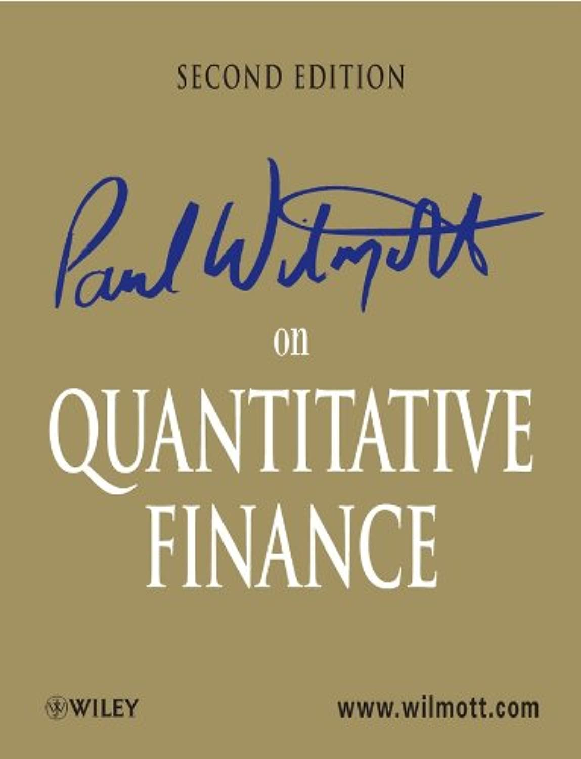
A trinomial model for the random walk

Untitled

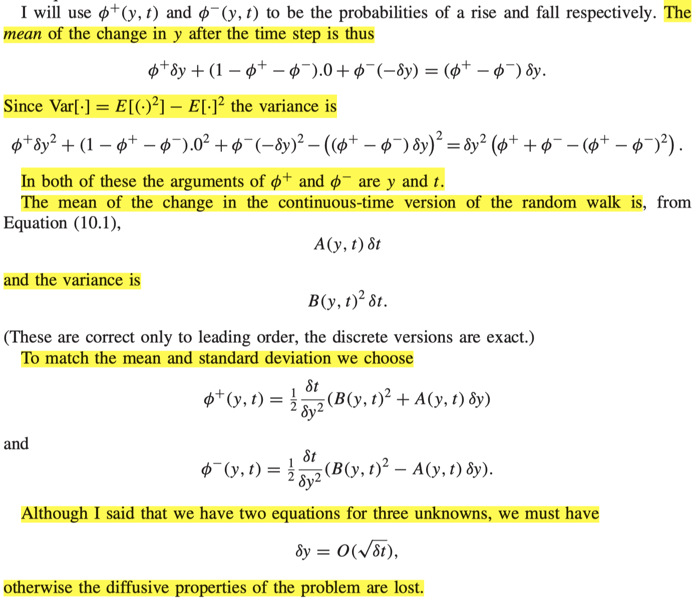
Rise and fall to be the same with probabilities such that the mean and standard deviation of the discrete-time approximation are the same as the mean and standard deviation of the continuous-time model over the same time step.

Jump size is $\delta y$, the probability of a rise and the probability of a fall, but only 2 quantities to fix, the mean and standard deviation

Untitled

The forward equation

Untitled

$$\frac{\partial p}{\partial t^{\prime }}=\frac{1}{2}\frac{{\partial }^2}{\partial y^{\prime 2}}(B(y^{\prime },t^{\prime }{)}^{2}p))-\frac{\partial }{\partial y^{\prime }}(A(y^{\prime },t^{\prime })p)$$

This is the Fokker-Planck or forward Kolmogorov equation.

• It is a forward parabolic partial differential equation, requiring initial conditions at time t and to be solved for t’ > t
• This equation is to be used if there is some special state now and you want to know what could happen later. For example, you know the current value of y and want to know the distribution of values at some later date.

Example

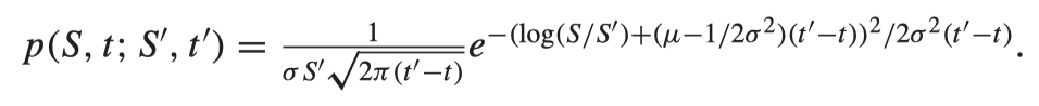
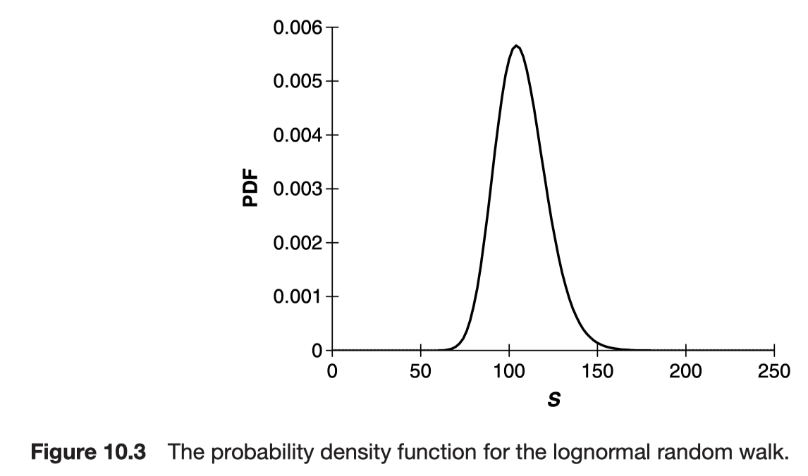
The distribution of equity prices in the future

$$dS=\mu Sdt+\sigma SdX$$

the forward equation becomes

$$\frac{\partial p}{\partial t^{\prime }}=\frac{1}{2}\frac{{\partial }^2}{\partial S^{\prime 2}}({\sigma }^2{S}^{\prime 2}p)-\frac{\partial }{\partial S^{\prime }}(\mu S^{\prime }p)$$

The solution is

Untitled

Untitled

The steady-state distribution

Steady-state distribution

• In the long run as $t^{\prime }\to \mathrm{\infty }$ the distribution p(y, t; y’, t’) as a function of y’ settles down to be independent of the starting state y and time t.
• This requires at least that the random walk is time homogeneous, i.e. that A and B are independent of t, asymptotically.

Untitled

If there is a steady-state distribution $p_{\mathrm{\infty }}(y^{\prime })$ then it satisfies

$$\frac{1}{2}\frac{d^2}{d{y}^{\prime 2}}(B_{\mathrm{\infty }}^2{p}_{\mathrm{\infty }})-\frac{d}{d{y}^{\prime }}(A_{\mathrm{\infty }}{p}_{\mathrm{\infty }})=0$$

$A_{\mathrm{\infty }}$ and $B_{\mathrm{\infty }}$ are the functions in the limit $t\to \mathrm{\infty }$

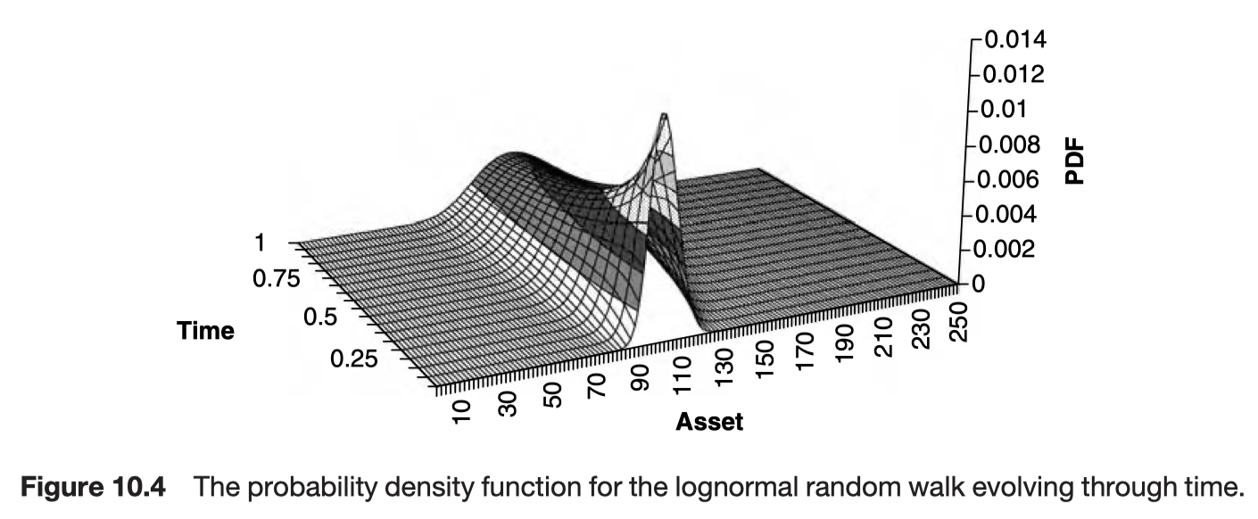
The backward equation

This will be useful if we want to calculate probabilities of reaching a specified final state from various initial states. It will be a backward parabolic partial differential equation requiring conditions imposed in the future, and solved backwards in time.

Untitled

Backward Kolmogorov equation

$$\frac{\partial p}{\partial t}+\frac{1}{2}B(y,t{)}^2\frac{{\partial }^{2}p}{\partial y^2}+A(y,t)\frac{\partial p}{\partial y}=0$$

First-exit times

The first-exit time is the time at which the random variable reaches a given boundary.

Untitled

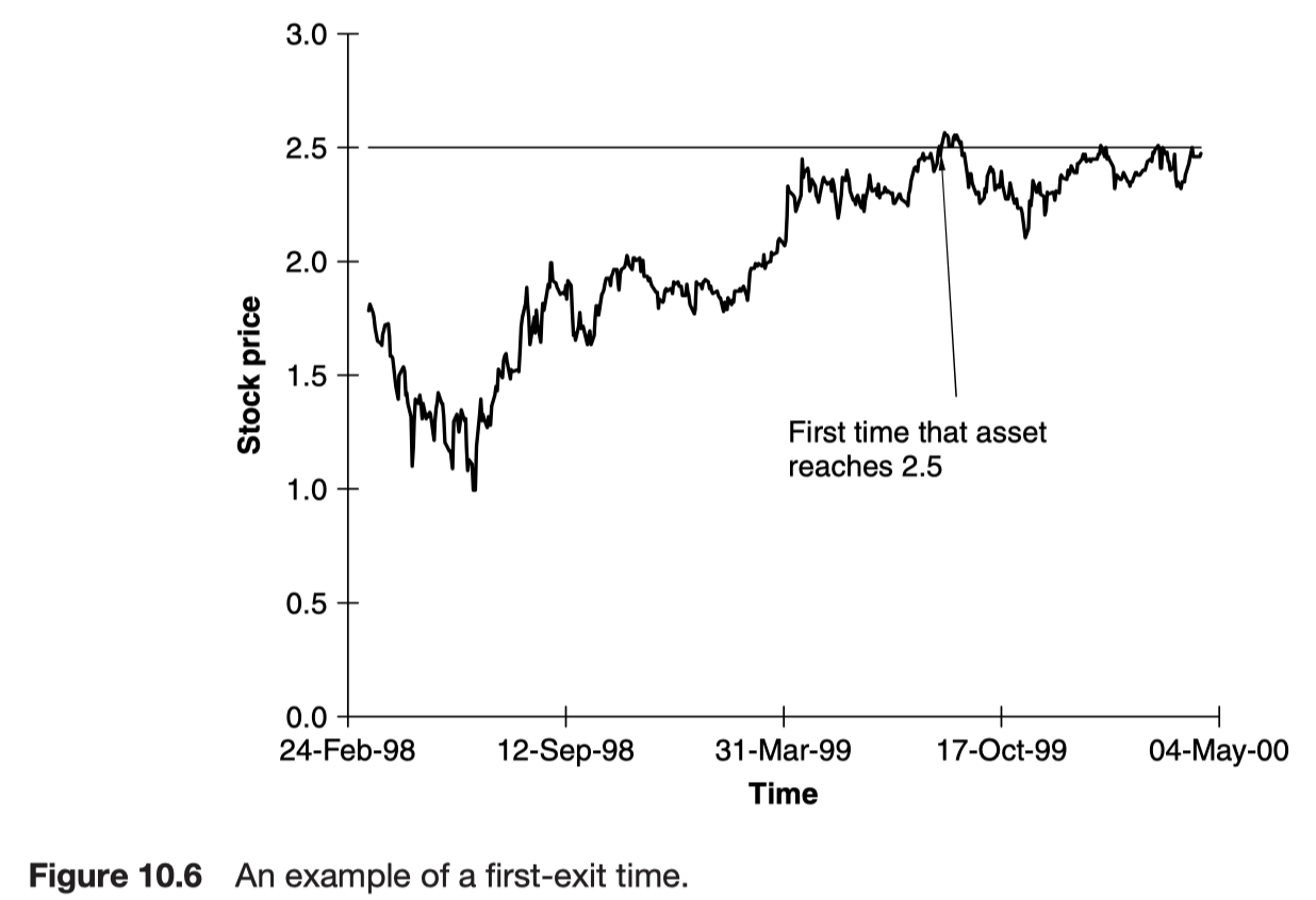
What is the probability of an asset level being reached before a certain time?

How long do you expect it to take for an interest rate to fall to a given level?

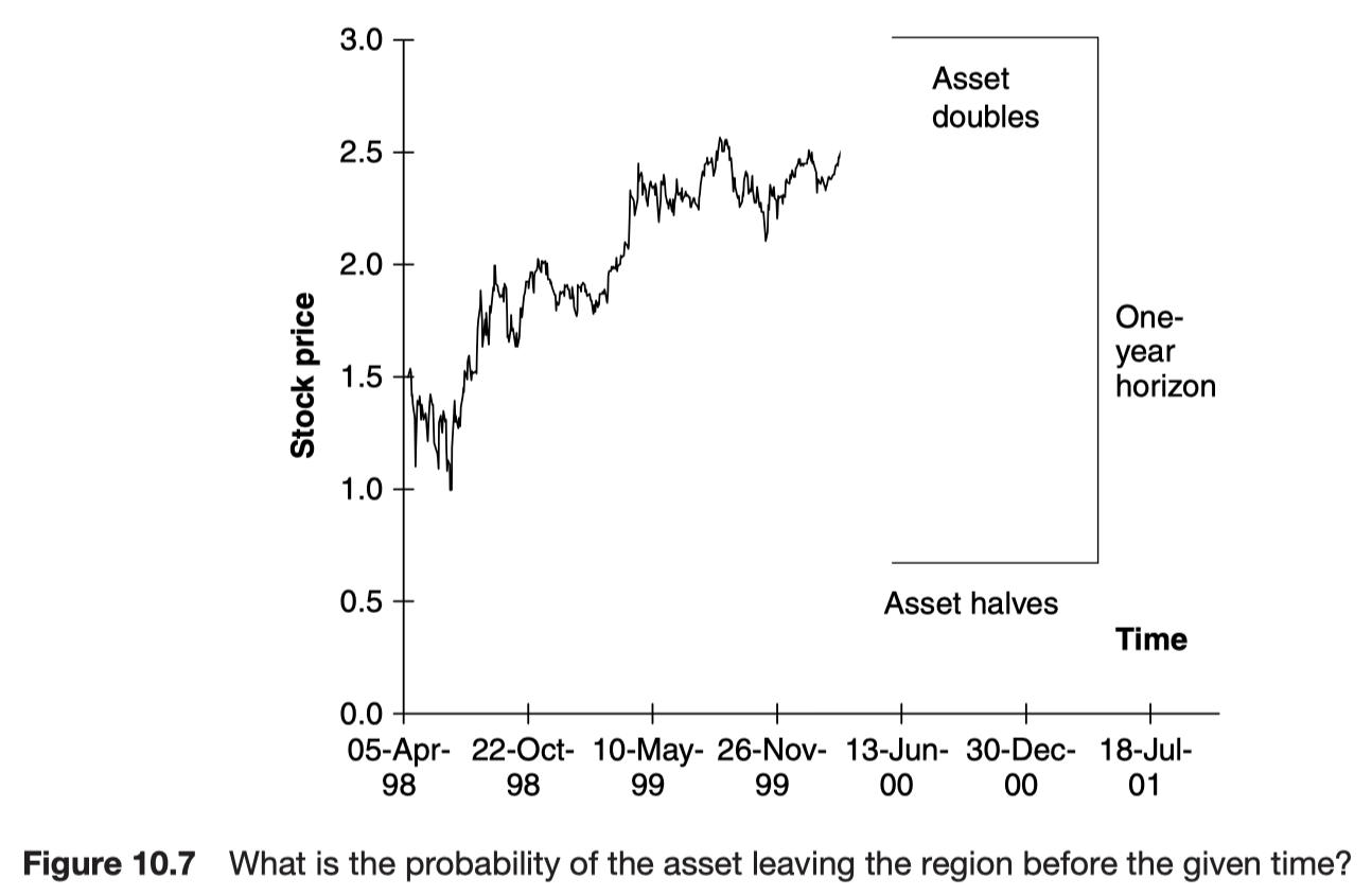
Cumulative distribution functions for first-exit times

What is the probability of your favorite asset doubling or halving in value in the next year?

What is the probability of a random variable leaving a given range before a given time?

$$\frac{\partial C}{\partial t}+\frac{1}{2}B(y,t{)}^2\frac{{\partial }^{2}C}{\partial y^2}+A(y,t)\frac{\partial C}{\partial y}=0$$

$$C(y,t:t^{\prime })$$

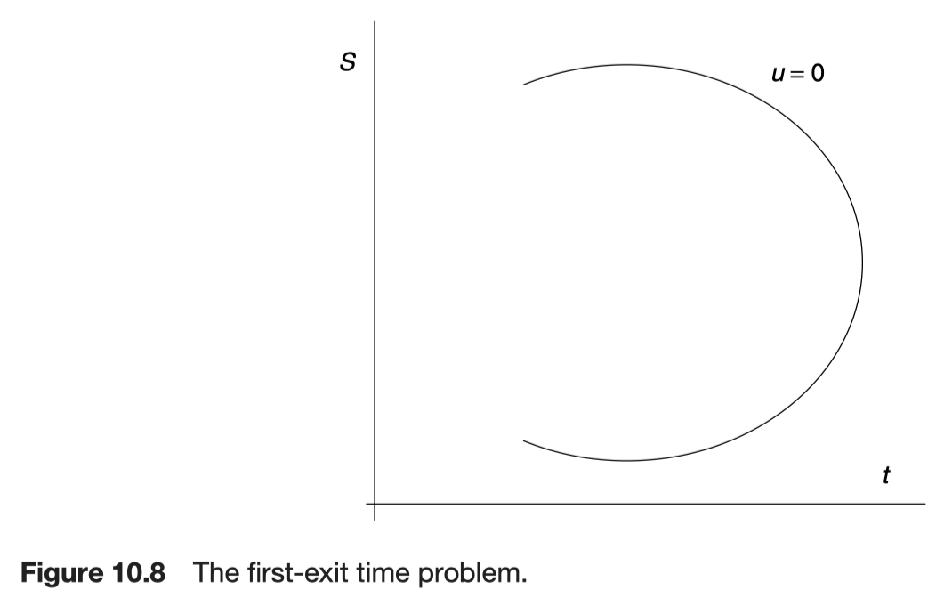
Function C is the probability of the variable y leaving the region $\mathrm{\Omega }$ before time t’. This function can be thought of as a cumulative distribution function.

What makes the problem different from that for the transition probability density function are the boundary and final conditions. If the variable y is actually on the boundary of the region $\mathrm{\Omega }$ then clearly the probability of exiting is one

$$C(y,t,t^{\prime })=1\text{on the edge of }\mathrm{\Omega }$$

On the other hand, if we are inside the region $\mathrm{\Omega }$ at time t’, then there is no time left for the variable to leave the region and so the probabiilty is zero.

$$C(y,t^{\prime },t^{\prime })=0$$

Untitled

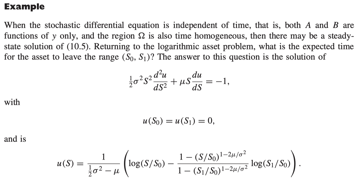
Expected first-exit times

expected first-exit time u(y, t)

$$u(y,t)={\int }_t^{\mathrm{\infty }}(t^{\prime }-t)\frac{\partial C}{\partial t^{\prime }}d{t}^{\prime }$$

$$u(y,t)={\int }_t^{\mathrm{\infty }}1-C(y,t;t^{\prime })d{t}^{\prime }$$

The function C satisfies the backward equation in y and t

$$\frac{\partial C}{\partial t}+\frac{1}{2}B(y,t{)}^2\frac{{\partial }^{2}C}{\partial y^2}+A(y,t)\frac{\partial C}{\partial y}=-1$$

Since C is one on the boundary of $\mathrm{\Omega }$, u must be zero around the boundary of the region.

Untitled

Untitled

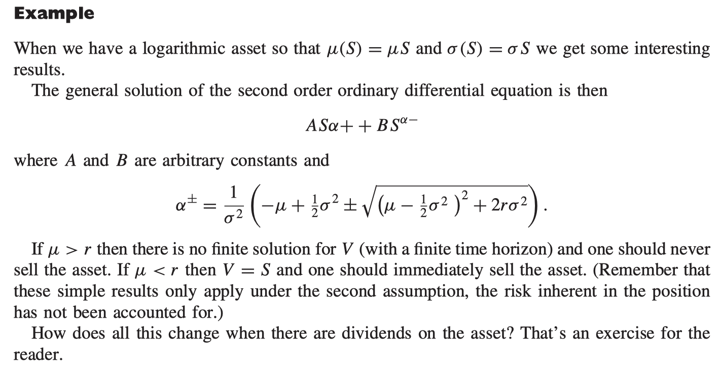
Another example of optimal stopping

Timing to sell - 2 assumptions

1. Knowing the statistical/stochastic properties of investment value

$$dS=\mu (S)dt+\sigma (S)dX$$

1. Wanting to sell at the time which maximize the expected value of investment, with suitable allowance being taken for the time value of money

$$\frac{1}{2}\sigma (S{)}^2\frac{d^{2}V}{d{S}^2}+\mu (S)\frac{dV}{dS}-rV=0$$

The last term on the left is the usual time-value-of-money term

This must be solved subject to

$$V\ge S$$

with continuity of V and dV/dS. This constraint ensures that we maximize our expected value.

Untitled

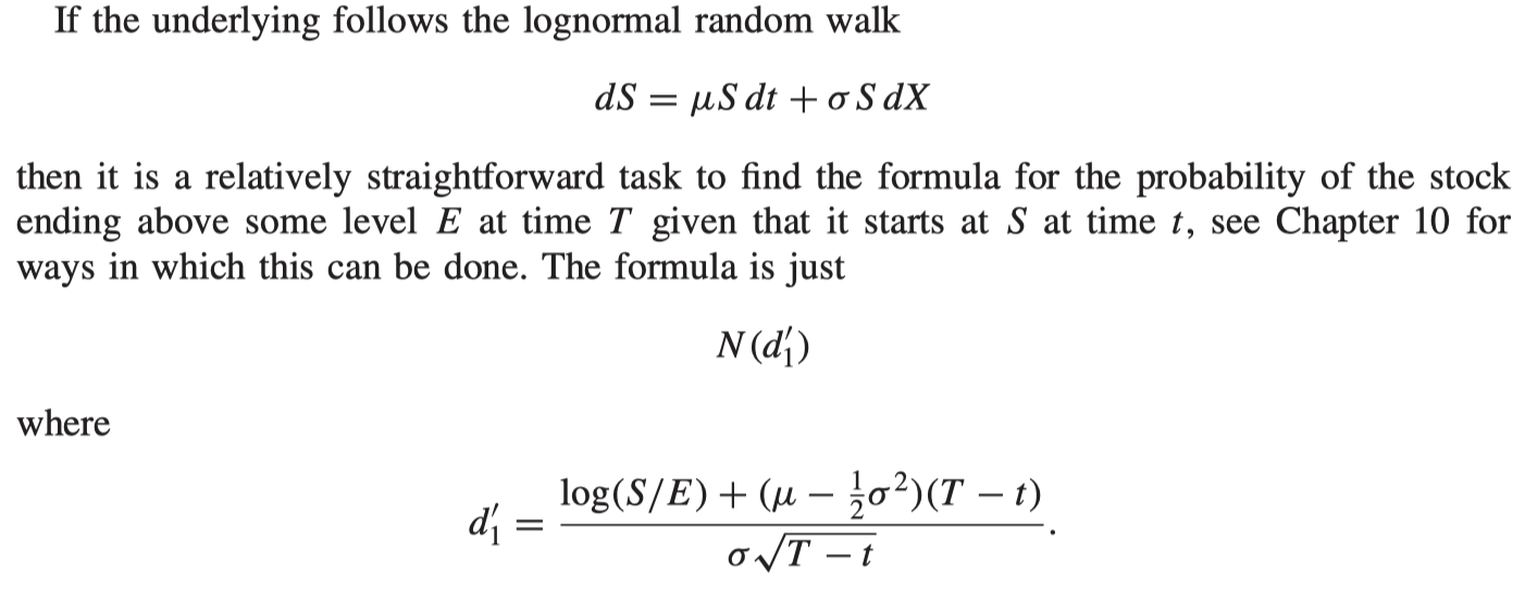
Expectations and Black-Scholes

$$dS=\mu Sdt+\sigma SdX$$

$$\frac{\partial p}{\partial t}+\frac{1}{2}{\sigma }^2{S}^2\frac{{\partial }^{2}p}{\partial S^2}+\mu S\frac{\partial p}{\partial S}=0$$

Expected value of some function F(S)

$$p_F(S,T)=F(S)$$

Present value of the expected amount of an option’s payoff

$$e^{-r(T-t)}{p}_F(S,t)$$

$$P_F(S,t)=e^{r(T-t)}V(S,t)$$

$$\frac{\partial V}{\partial t}+\frac{1}{2}{\sigma }^2{S}^2\frac{{\partial }^{2}V}{\partial S^2}+\mu S\frac{\partial V}{\partial S}-rV=0$$

$$dS=\mu Sdt+\sigma SdX$$

This is called the risk-neutral random walk.

The fair value of an option is the present value of the expected payoff at expiry under a risk-neutral random walk for the underlying.

$$\text{option value}=e^{-r(T-t)}E[payoff(S)]$$

provided that the expectation is with respect to the risk-neutral random walk, not the real one.

This result is the main contribution to finance theory of what is known as the martingale approach to pricing.

A common misconception

Untitled

Delta is not the probability of an option ending up in the money. The 2 reasons are

1. There is a $\mu$ in the formula for the probability. There is no $\mu$ in the option’s delta. We want to know what the real probability of ending up in the money is, and option prices have nothing to do with real probabilities.
2. There is a sign difference.

Summary

If you own an American option when do you expect to exercise it? The value depends theoretically on the parameter $\sigma$ in the asset price random walk but the expected time to exercise also depends on $\mu$; the payoff may be certain because of hedging but you cannot certain whether you will still hold the option at expiry.

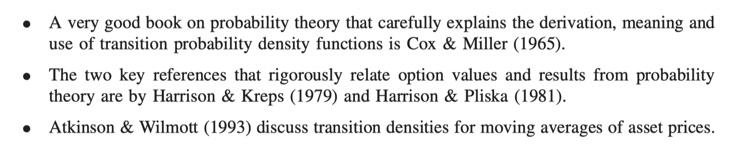
Further reading

Untitled

Untitled.png