Quantitative Finance - Chapter 12 - how to delta hedge

Untitled.png

• how to make money if your volatility is more accurate than the market’s
• different ways of delta hedging
• how much profit should you expect to make

Introduction

There is money to be made from options because options may be mispriced by the market. There are arbitrage opportunities.

Bet on actual volatility and implied volatility have different risk/return profiles.

Untitled

What if implied and actual volatilities are different?

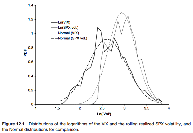
Actual volatility is the amount of ‘noise’ in the stock price; it is the coefficient of the Winer process in the stock returns model; it is the amount of randomness that ‘actually’ transpires. Implied volatility is how the market is pricing the option currently.

If you buy an at-the-money straddle close to expiry, the profit you expect to make from this strategy is approximately

$$\sqrt{\frac{2(T-t)}{\pi }}(\sigma -\tilde{\sigma })S$$

The standard deviation of the profit (the risk) is approximately

$$\sqrt{1-\frac{2}{\pi }}\sigma S\sqrt{T-t}$$

The standard deviation depends on the actual volatility only.

Implied versus actual; delta hedging but using which volatility?

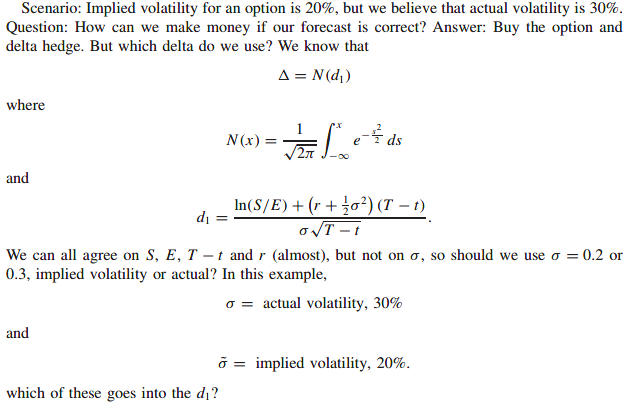
Which delta do you choose? actual or implied?

Untitled

Case 1: hedge with actual volatility, $\sigma$

By hedging with actual volatility we are replicating a short position in a correctly priced option. The payoffs for our long option and our short replicated option will exactly cancel. The profit will be exactly the difference in the Black-Scholes prices of an option with 30% volatility and one with 20% volatility.

$$V(S,t;\sigma )-V(S,t;\tilde{\sigma })$$

$$dS=\mu Sdt+\sigma SdX$$

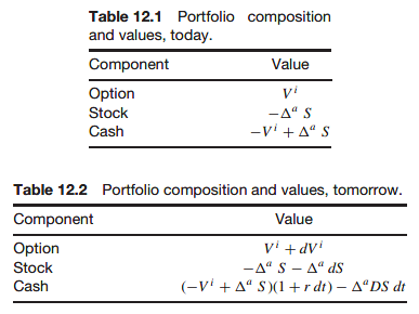
Set up a portfolio by buying the option for $V^i$ and hedge with ${\mathrm{\Delta }}^a$ of the stock.

Mark to market

$$d{V}^i-{\mathrm{\Delta }}^{a}dS-r(V^i-{\mathrm{\Delta }}^{a}S)dt-{\mathrm{\Delta }}^{a}DSdt$$

Since the option would be correctly valued at $V^a$,

$$d{V}^a-{\mathrm{\Delta }}^{a}dS-r(V^a-{\mathrm{\Delta }}^{a}S)dt-{\mathrm{\Delta }}^{a}DSdt=0$$

Untitled

mark-to-market profit over one time step as

$$d{V}^i-d{V}^a+r(V^a-{\mathrm{\Delta }}^{a}S)dt-r(V^i-{\mathrm{\Delta }}^{a}S)dt=d{V}^i-d{V}^a-r(V^i-V^a)dt=e^{rt}d(e^{-rt}(V^i-V^a))$$

The present value of this profit at time $t_0$ is

$$e^{-r(t-t_0)}{e}^{rt}d(e^{-rt}(V^i-V^a))=e^{r{t}_0}d(e^{-rt}(V^i-V^a))$$

So the total profit from $t_0$ to expiration is

$$e^{r{t}_0}{\int }_{t_0}^{T}d(e^{-rt}(V^i-V^a))=V^a-V^i$$

Untitled

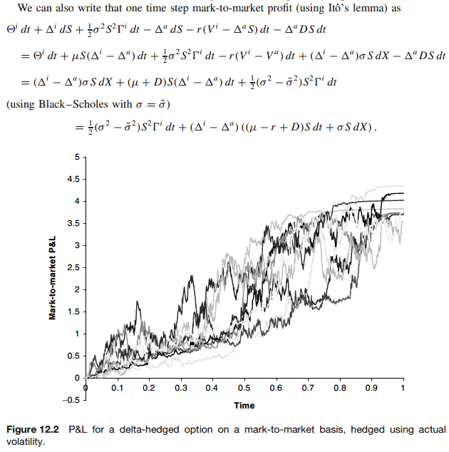
The conclusion is that the final profit is guaranteed but how that is achieved is random, because of the dX term in the above. On a mark-to-market basis you could lose before you gain. Moreover, the mark-to-market profit depends on the real drift of the stock, $\mu$.

When S changes, so will V. But these changes do not cancel each other out. From a risk management point of view this is not ideal.

It is similar to owning a bond. For a bond there is a guaranteed outcome, but we may lose on a mark-to-market basis in the meantime.

Case 2: hedge with implied volatility, $\tilde{\sigma }$

By hedging with implied volatility we are balancing the random fluctuations in the mark-to-market option value with the fluctuations in the stock price. The evolution of the portfolio value is then ‘deterministic.’

The mark-to-market profit from today to tomorrow is

$$d{V}^i-{\mathrm{\Delta }}^{i}dS-r(V^i-{\mathrm{\Delta }}^{i}S)dt-{\mathrm{\Delta }}^{i}DSdt={\mathrm{\Theta }}^{i}dt+\frac{1}{2}{\sigma }^2{S}^2{\mathrm{\Gamma }}^{i}dt-r(V^i-{\mathrm{\Delta }}^{i}S)dt-{\mathrm{\Delta }}^{i}DSdt=\frac{1}{2}({\sigma }^2-{\tilde{\sigma }}^2)S^2{\mathrm{\Gamma }}^{i}dt$$

The daily profit is deterministic, there aren’t any dX term. From a risk management perspective this much better behaved.

We don’t even need to know what actual volatility is. And to make a profit all we need to know is that actual is always going to be greater than implied (if we are buying) or always less (if we are selling)

The present value of all of these profits to get a total profit of

$$\frac{1}{2}({\sigma }^2-{\tilde{\sigma }}^2){\int }_{t_0}^T{e}^{-r(t-t_0)}{S}^2{\mathrm{\Gamma }}^{i}dt$$

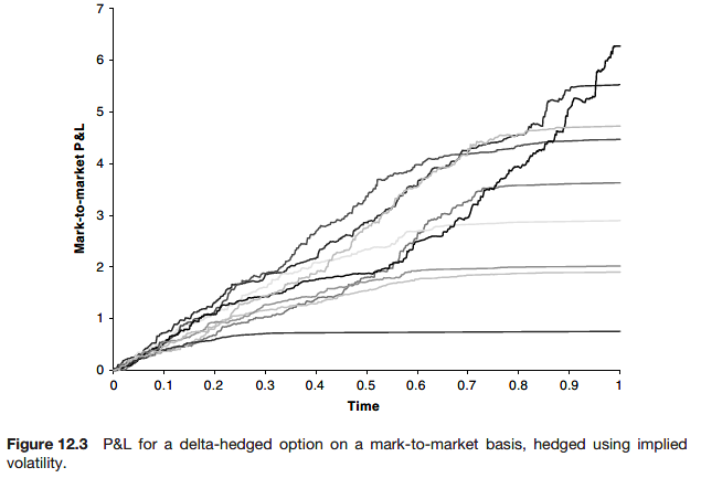
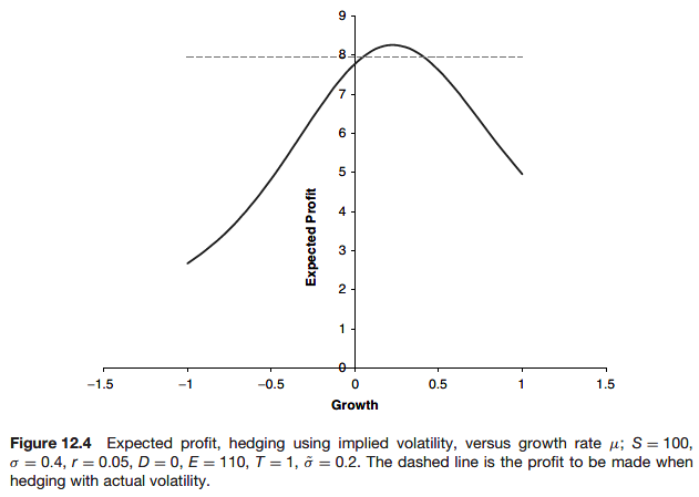
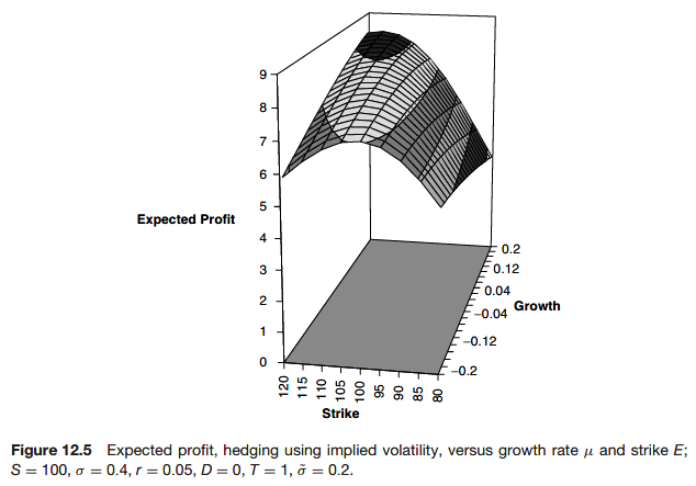
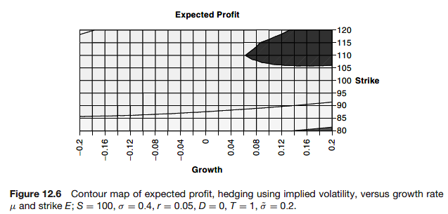
This is always be positive, but highly path dependent. Being path dependent it will depend on the drift $\mu$.

Untitled

Peter Carr (2005) and Henrard (2001) show that if you hedge using a delta based on a volatility ${\sigma }_h$ then the PV of the total profit is given by

$$V(S,t;{\sigma }_h)-V(S,t;\tilde{\sigma })+\frac{1}{2}({\sigma }^2-{\sigma }_h^2){\int }_{t_0}^T{e}^{-r(t-t_0)}{S}^2{\mathrm{\Gamma }}^{h}dt$$

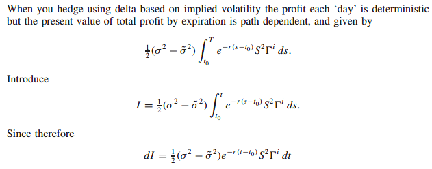
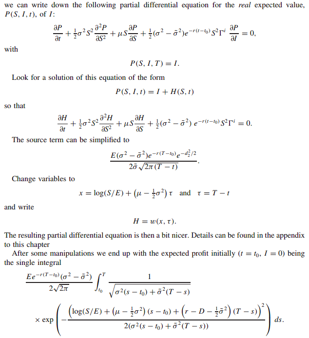
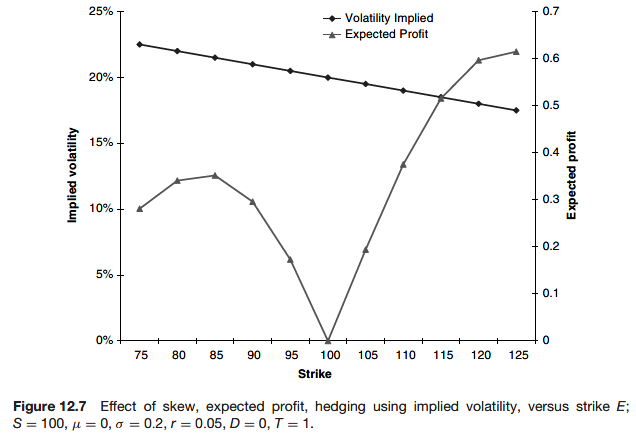
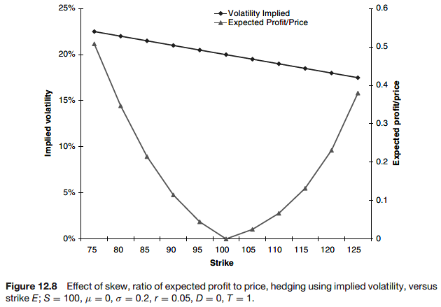
The expected profit after hedging using implied volatility

Untitled

Untitled

Untitled

Untitled

Untitled

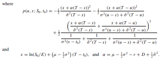
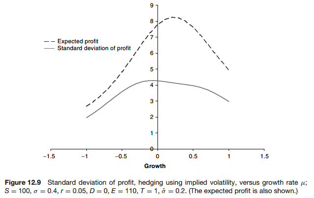
The variance of profit after hedging using implied volatility

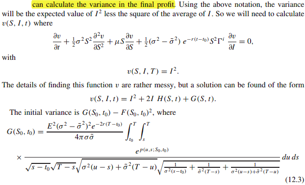
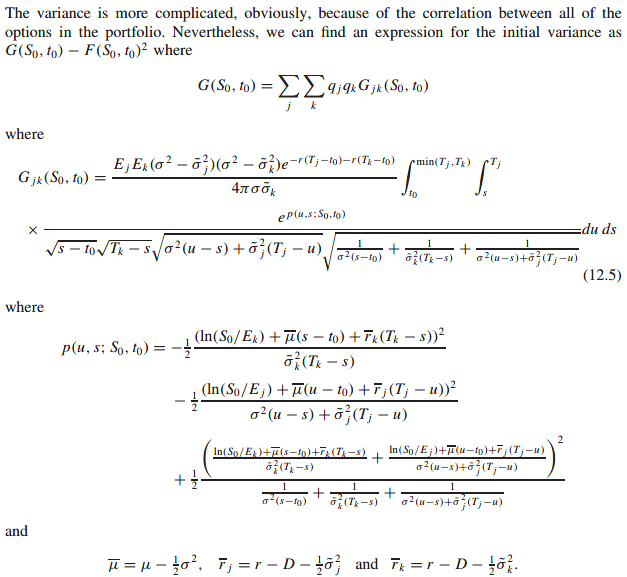
Once we have calculated the expected profit from hedging using implied volatility we can calculate the variance in the final profit.

Untitled

Untitled

Untitled

Untitled

Untitled

Untitled

Untitled

Untitled

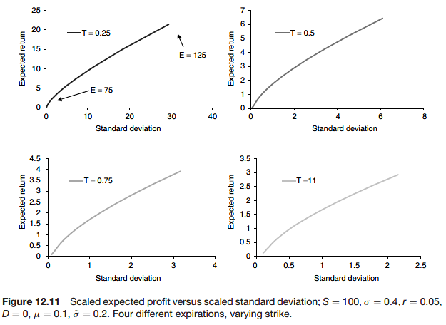
Hedging with different volatilities

Untitled

Untitled

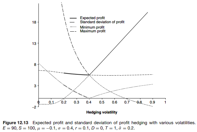
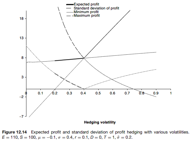
In this case, it is more usual to hedge based on implied volatility to avoid the daily fluctuations in the profit and loss.

Portfolios when hedging with implied volatility

Since only an option’s gamma matters when we are hedging using implied volatility, calls and puts are effectively the same since they have the same gamma.

The profit from a portfolio is now

$$\frac{1}{2}\sum _k{q}_k({\sigma }^2-{\tilde{\sigma }}_k^2){\int }_{t_0}^{T_k}{e}^{-r(s-t_0)}{S}^2{\mathrm{\Gamma }}_k^{i}ds$$

where k is the index for an option, and $q_k$ is the quantity of that option. Introduce

$$I=\frac{1}{2}\sum _k{q}_k({\sigma }^2-{\tilde{\sigma }}_k^2){\int }_{t_0}^{T_k}{e}^{-r(s-t_0)}{S}^2{\mathrm{\Gamma }}_k^{i}ds$$

as a new state variable.

The governing differential operator for expectation, variance, etc. is then

$$\frac{\partial }{\partial t}+\frac{1}{2}{\sigma }^2{S}^2\frac{{\partial }^2}{\partial S^2}+\mu S\frac{\partial }{\partial S}+\frac{1}{2}\sum _k({\sigma }^2-{\tilde{\sigma }}_k^2)e^{-r(t-t_0)}{S}^2{\mathrm{\Gamma }}_k^i\frac{\partial }{\partial I}=0$$

Expectation

Untitled

Variance

Untitled

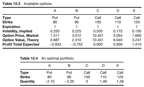
Portfolio optimization possibilities

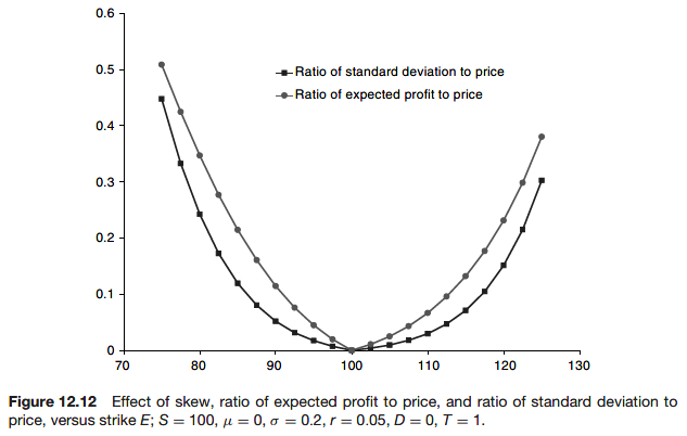
Observe the negative skew. The out-of-the-money puts are overvalued and the out-of-the-money calls are undervalued.

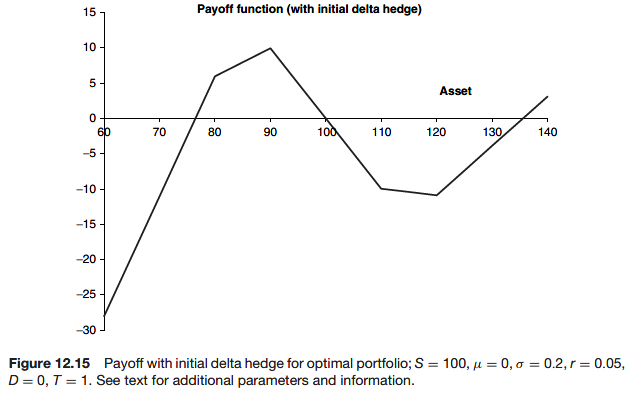
Using the above formulae we can find the portfolio that maximizes or minimizes target quantities.

This is a very natural strategy when trying to make a profit from volatility arbitrage while meeting constraints imposed by regulators, brokers, investors etc.

Untitled

Untitled

Hedging when implied volatility is stochastic

$$d\tilde{\sigma }=adt+bd{X}_2$$

with random component $d{X}_1$ and actual volatility constant.

There will be a correlation coefficient between $d{X}_1$ and $d{X}_2$ of $\rho$.

Case 1: hedge with actual volatility, $\sigma$

The argument that the final profit is guaranteed is not affected by having implied volatility stochastic, except insofar as you may get the opportunity to close the position early if implied volatility reaches the level of actual.

Untitled

Case 2: hedge with implied volatility, $\tilde{\sigma }$?

It is not clear that using the delta based on implied volatility is meaningful when implied volatility is stochastic.

Untitled

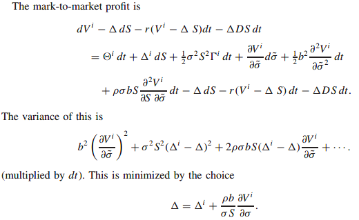
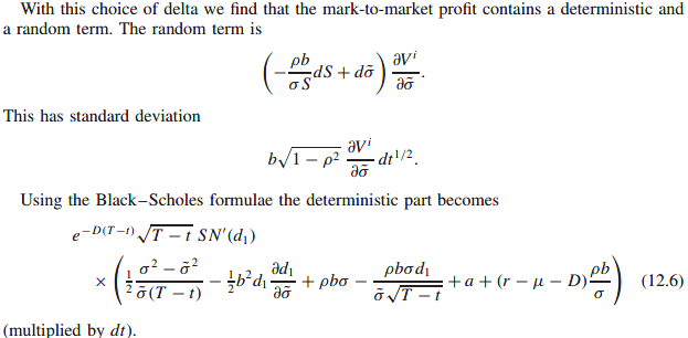
This confirms that to minimize risk on a mark-to-market basis you must adjust delta by the vega.

Untitled

How does implied volatility behave?

What does it mean for making money if we think that the market if wrong?

Sticky strike

In this model implied volatility remains constant for each option. As far as making a profit if the implied volatility is different from actual volatility.

Sticky delta

Since the delta of an option is a function of its moneyness, S/E, the sticky delta behavior could also be called the sticky moneyness rule. This behavior is commonly seen in the FX markets, possibly because there it is usual to quote option prices/volatilities for options with specific deltas rather than specific strike.

$$\tilde{\sigma }=g(S/E,t)$$

$$d\tilde{\sigma }=(\frac{\partial g}{\partial t}+\mu \frac{S}{E}\frac{\partial g}{\partial \xi }+\frac{1}{2}{\sigma }^2\frac{S^2}{E^2}\frac{{\partial }^{2}g}{\partial {\xi }^2})dt+\sigma \frac{S}{E}\frac{\partial g}{\partial \xi }d{X}_1,\xi =S/E$$

The most important point about this expression is that it is perfectly correlated with dS, $\rho =1$, so that perfect hedging (in the mark-to-market sense) is possible.

A variation on this theme is to have implied volatility at different strikes being proportional to the ATM volatility and a function of the moneyness.

$$\tilde{\sigma }={\sigma }_{ATM}g(\frac{\log (S/E)}{\sqrt{T-t}})$$

Time-periodic behavior

Untitled

Untitled

Untitled

Untitled

Further reading

Untitled