- the names and properties of the basic and most important fixed-income products
- the definitions of features commonly found in fixed-income products
- simple ways to analyze the market value of the instruments: yield, duration and convexity
- how to construct yield curves and forward rates
Simple fixed-income contracts and features
The zero-coupon bond
The zero-coupon bond is a contract paying a known fixed amount, the principal, at some given date in the future, the maturity date T.
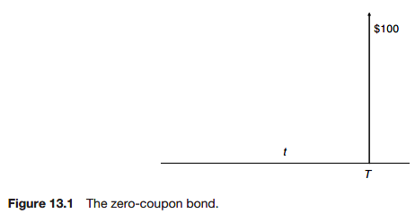
It cannot have zero or negative value.
The coupon-bearing bond
The coupon-bearing bond is similar to the zero-coupon bond except that as well as paying the principal at maturity, it pays smaller quantities, the coupons, at intervals up to the including the maturity date.
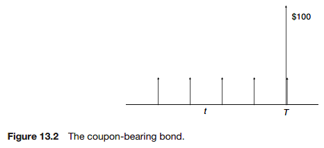
These coupons are usually prespecified fractions of the principal.
We can think of the coupon-bearing bond as a portfolio of zero-coupon bearing bonds; one zero-coupon bearing bond for each coupon date with a principal being the same as the original bonds’ coupon, and then a final zero-coupon bond with the same maturity as the original.
The money market account
This is an account that accumulates interest compounded at a rate that varies from time to time. The rate at which interest accumulates is usually a short-term and unpredictable rate.
Floating rate bonds
The amount varies from time to time, reflecting the state of the economy and in response to pressure from other banks for your business.
The most common measure of interest is London Interbank Offer Rate or LIBOR. LIBOR comes in various maturities and is the rate of interest offered between Eurocurrency banks for fixed-term deposits.
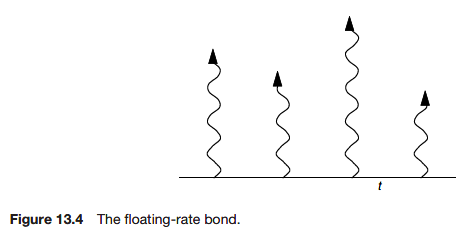
Sometimes the coupon payment on a bond is not a prescribed dollar amount but depends on the level of some ‘index’, measured at the time of the payment or before.
Forward rate agreements
A Forward rate agreement (FRA) is an agreement between two parties that a prescribed interest rate will apply to a prescribed principal over some specified period in the future.
Repos
A repo is a repurchase agreement. It is an agreement to sell some security to another party and buy it back at a fixed date and for a fixed amount. The price at which the security is bought back is greater than the selling price and the difference implies an interest rate called the repo rate. The commonest repo is the overnight repo in which the agreement is renegotiated daily. If the repo agreement extends for 30 days it is called a term repo.
A reverse repo is the borrowing of a security for a short period at an agreed interest rate.
Repos can be used to lock in future interest rates.
- repo - sell and buy back
- reverse repo - buy and sell back
In repo transaction
- repo ↔︎ reverse repo
STRIPS
STRIPS stands for ‘Separate Trading of Registered Interest and Principal of Securities’. The coupons and principal of normal bonds are split up.
Amortization
All of the above products are assumed that the principal remains fixed at its initial level.
The principal can amortize or decrease during the life of the contract. The principal is thus paid back gradually and interest is paid on the amount of the principal outstanding. Such amortization is arranged at the initiation of the contract and may be fixed, so that the rate of decrease of the principal is known beforehand, or can depend on the level of some index.
Call provision
The issuer can call back the bond on certain dates or at certain periods for a prescribed, possibly time-dependent, amount.
International bond markets
United States of America
maturity
- bills - less than 1 year, zero-coupon bond
- notes - 2-10 years
- bonds - greater than 10 years
Bond traded in the US foreign bond market but which are issued by non-US institutions are called Yankee bonds.
Since the beginning of 1997 the US government has also issued bonds linked to the rate of inflation.
United Kingdom
Bond issued by the UK government are called gilts.
Some of these bonds are callable, some are irredeemable, meaning that they are perpetual bonds having a coupon but no repayment of principal. The government also issues convertible bonds which may be converted into another bond issue, typically of longer maturity.
There are index-linked bonds having the amount of the coupon and principal payments linked to a measure of inflation, the Retail Price Index (RPI).
Japan
Japanese Government Bonds (JGBs)
- short-term treasury bills, zero-coupon
- medium-term, long-term: 10-year maturity, semi-annual
- super long-term: 20-year maturity, semi-annual
Yen denominated bonds issued by non-Japanese institutions are called Samurai bonds.
Accrued interest
The market price of bonds quoted are clean price. That is, they are quoted without any accrued interest.
The accrued interest is the amount of interest that has build up since the last coupon payment:
\[ \text{accrued interest} = \text{interest due in full period} \times \frac{\text{number of days since last coupon date}}{\text{number of days in period between coupon payments}} \]
The actual payment is called the dirty price and is the sum of the quoted clean price and the accrued interest.
Day-count conventions
\[ \frac{\text{number of days between two dates}}{\text{number of days in period}} \times \text{interest earned in reference period} \]
- Actual/Actual
- 30/360
- Actual/360
Continuously and discretely compounded interest
present value with continuously compounded rate
\[ e^{-rT} \]
money market account equation
\[ dM = rMdt \]
This is the convention used in the options world.
present value with discretely compounded rate
\[ \frac{1}{(1 + r')^T} \]
The relationship between the continuously compounded interest rate r and the discrete version r’
\[ r = \log{(1 + r')} \]
Measures of yield
Through measures of how much each contract earns; there are several measures of this all coming under the name yield.
Current yield
\[ \text{current yield} = \frac{\text{annual coupon income}}{bond price} \]
It is concentrating very much on short-term properties of the bond.
The yield to maturity (YTM) or interest rate of return (IRR)
\[ Z(t; T) = e^{-r(T - t)} \]
\[ y = -\frac{\log Z}{T - t} \]
The present value of the bond at time t
\[ V = Pe^{-r(T - t)} + \sum_{i = 1}^N{C_i e^{-y(t_i - t)}} \]
The value y is the yield to maturity or internal rate of return.
This YTM is a valid measure of the return on a bond if we intend to hold it to maturity.
To calculate YTM of a portfolio of bonds simply treat all the cashflows as if they were from the one bond and calculate the value of the whole portfolio by adding up the market values of the component bonds.
The yield curve
The plot of YTM against time to maturity is called the yield curve.
For the moment assume that this has been calculated from zero-coupon bonds and that these bonds have been issued by a perfectly creditworthy source.
Price/yield relationship

Duration
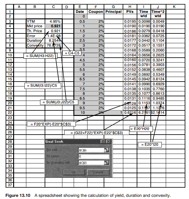
\[ \frac{dV}{dy} = -(T - t)Pe^{-r(T - t)} - \sum_{i = 1}^N{C_i(t_i - t)e^{-y(t_i - t)}} \]
Macaulay duration
\[ -\frac{1}{V}\frac{dV}{dy} \]
Modified duration
\[ \text{modified duation} = \frac{\text{Macaulay duration}}{1 + YTM} \]
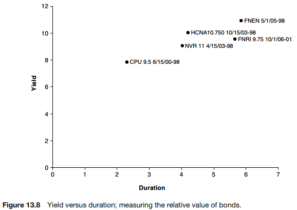
The duration is a measure of the average life of the bond.
What maturity would an ‘equivalent’ bond have?
\[ V = Pe^{-r(T - t)} + \sum_{i = 1}^N{C_i e^{-y(t_i - t)}} = Xe^{-r(\bar T - t)} \]
\[ \frac{dV}{dy} = -(T - t)Pe^{-r(T - t)} - \sum_{i = 1}^N{C_i(t_i - t)e^{-y(t_i - t)}} = -X (\bar T - t)e^{-y(\bar T - t)} \]
\[ -\frac{1}{V}\frac{dV}{dy} = \dots = \bar T - t \]
For small movements in the yield, the duration gives a good measure of the change in value with a change in the yield. For larger movements we need to look at higher order terms in the Taylor series expansion of V(y).
Convexity
The Taylor series expansion of V gives
\[ \frac{dV}{V} = \frac{1}{V}\frac{dV}{dy}\delta y + \frac{1}{2V}\frac{d^2 V}{dy^2}(\delta y)^2 + \dots \]
where \(\delta y\) is a change in yield.
the dollar convexity
\[ \frac{d^2 V}{dy^2} = (T - t)P^{-r(T - t)} + \sum_{i = 1}^N{C_i(t_i - t)^2e^{-r(t_i - t)}} \]
The convexity is
\[ \frac{1}{V}\frac{d^2 V}{dy^2} \]

When we develop a consistent theory for pricing bonds when interest rates are stochastic we will se how the absence of arbitrage will lead to relationships between such quantities as yield, duration and convexity, not unlike the Black-Scholes equation.
Hedging
\[ \Pi = V_A(y_A) - \Delta V_B(y_B) \]
Assume parallel shifts in the yield curve.
the change in the value of this portfolio is
\[ \delta\Pi = \frac{\partial V_A}{\partial y_A}x - \Delta \frac{\partial V_B}{\partial y_B} + \text{the higher-order terms} \]
The higher-order term depend on the convexity of the 2 instruments.
\[ \Delta = \frac{\partial V_A}{\partial y_A} / \frac{\partial V_B}{\partial y_B} \]
Time-dependent interest rate
The interest rate we consider will be what is known as a short-term interest rate or spot interest rate r(t). This means that the rate r(t) is to apply at time t; interest is compounded at this rate at each moment in time but this rate may change: generally we assume it to be time dependent.
If the spot interest rate r(t) is a known function of time, then the bond price is also a function of time only: V = V(t).
The change in the value of that bon din a time-step dt from t to t + dt is
\[ \frac{dV}{dt}dt \]
Arbitrage considerations again lead us to equate this with the return from a bank deposit receiving interest at a rate r(t):
\[ \frac{dV}{dt} = r(t)V \]
The solution of this equation is
\[ V(t; T) = e^{-\int_t^T{r(\tau)d\tau}} \]
If during the period t to t + dt we have received a coupon payment of K(t)dt, which may be either in the form of continuous or discrete payments or a combination, our holdings including cash change by an amount
\[ \left(\frac{dV}{dt} + K(t)\right)dt \]
Again setting this equal to the risk-free rate r(T) we conclude that
\[ \frac{dV}{dt} + K(t) = r(t)V \]
\[ V(t) = e^{-\int_t^T{r(\tau)d\tau}}\left(1 + \int_t^T{K(t')e^{\int_{t'}^T{r(\tau)d\tau}}dt'}\right) \]
the arbitrary constant of integration has been chosen to ensure that V(T) = 1.
Discretely paid coupons
Since the holder of the bond receives a coupon, call it \(K_c\), at time \(t_c\) there must be a jump in the value of the bond across the coupon date. That is, the values before and after this date differ by \(K_c\)
\[ V(t_c^-) = V(t_c^+) + K_c \]
This will be recognized as a jump condition. This time the realized bond price is not continuous.
Forward rates and bootstrapping
The main problem with the use of YTM as a measure of interest rates is that is not consistent across instruments.
One way of overcoming this problem is to use forward rates.
Forward rates are interest rates that are assumed to apply over given periods in the future for all instruments.
Let us suppose that we are in a perfect world in which we have a continuous distribution of zero-coupon bonds with all maturities T. Call the prices of these at time t, Z(t; T). Note the use of Z for zero-coupon.
The implied forward rate is the curve of a time-dependent spot interest rate that is consistent with the market price of instruments.
\[ Z(t; T) = e^{-\int_t^T{r(\tau)d\tau}} \]
On rearranging and differentiating this gives
\[ r(T) = -\frac{\partial}{\partial T}(\log{Z(t; T)}) \]
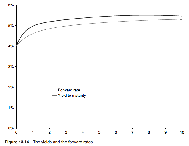
\[ F(t; T) = -\frac{\partial}{\partial T}(\log{Z(t; T)}) \]
\[ Z(t; T) = e^{-y(t; T)(T - t)} \]
\[ F(t; T) = y(t; T) + \frac{\partial y}{\partial T} \]
Discrete data
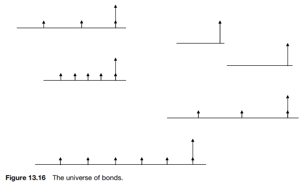
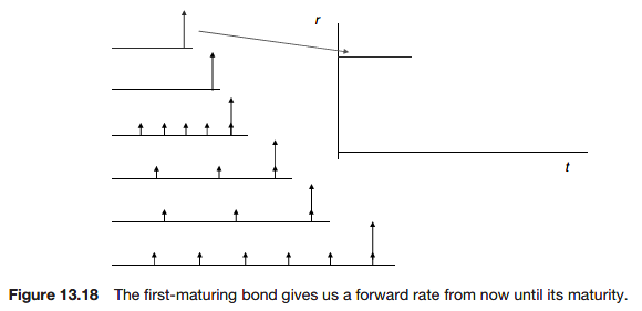
\[ Z_1^M = e^{-y_1(T_1 - t)} \]
\[ y_1 = -\frac{\log{(Z_1^M)}}{T_1 - t} \]
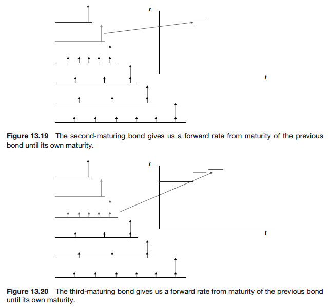
\[ Z_2^M = e^{-y_1(T_1 - t)}e^{-y_2(T_2 - T_1)} \]
\[ y_2 = -\frac{\log{(Z_2^M / Z_1^M)}}{T_2 - T_1} \]
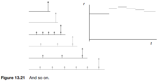
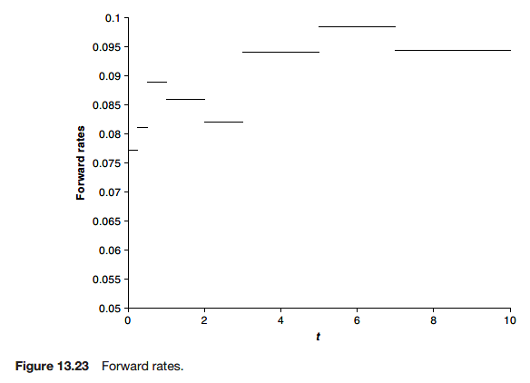
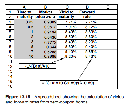
By this method of bootstrapping we can build up the forward rate curve.
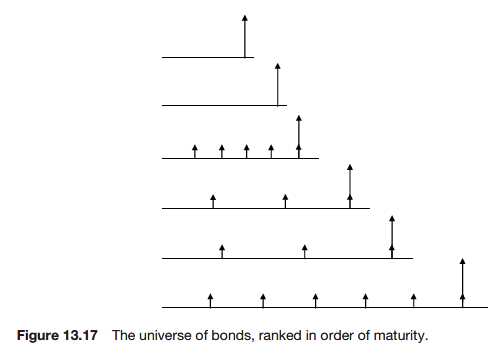

On a spreadsheet
Interpolation
We have explicitly assumed in the previous section that the forward rates are piecewise constant, jumping from one value to the next across the maturity of each bond. Other methods of ‘interpolation’ are also possible.
Further reading
