- a simple model for an asset price random walk
- delta hedging
- no arbitrage
- the basics of the binomial method for valuing options
- risk neutrality
Introduction
The binomial model is the more accessible version of Black-Scholes equation.
As a model of stock price behavior it is poor. The binomial model says that the stock can either go up by a known amount or down by a known amount.
Equities can go down as well as up
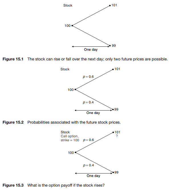
- call option on a stock, expiring tomorrow
- The stock can either rise or fall by a known amount between today and tomorrow
- Interest rates are zero

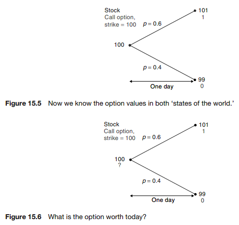
The option value
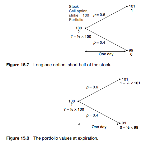
Which part of our ‘model’ didn’t we need?
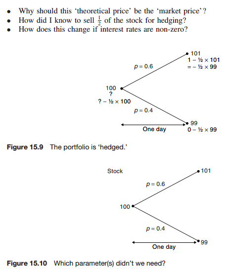
Why should this ‘theoretical price’ be the ‘market price’?
Because if it’s not, then there is risk-free money to be made.
The role of expectations
Unless the were risk seeking.
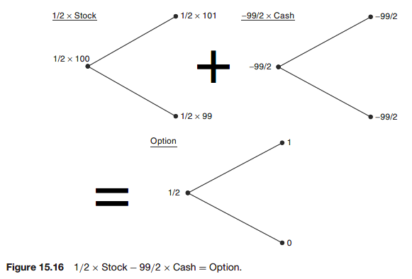
How did I know to sell 1/2 of the stock for hedging?
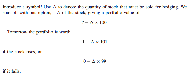

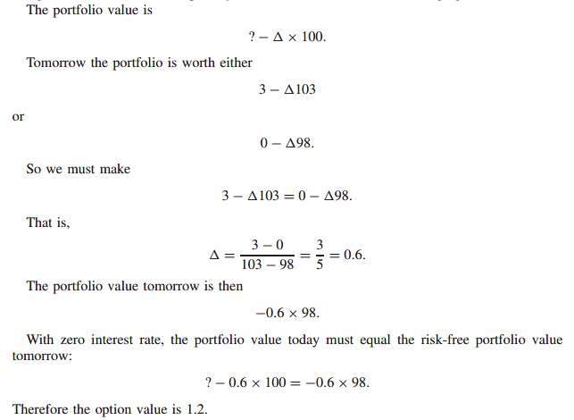
The general formula for \(\Delta\)
Delta hedging means choosing \(\Delta\) such that the portfolio value does not depend on the direction of the stock.
\[ \Delta = \frac{\text{range of option payoffs}}{\text{range of stock prices}} \]
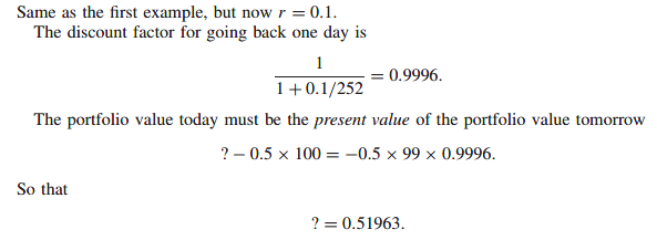
How does this change if interest rates are non-zero?
Is the stock itself correctly priced?
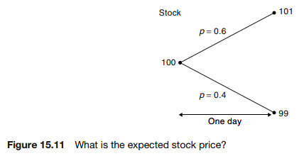

We pay less than the future expected value because the stock is risky. We want a positive expected return to compensate for the risk.
Complete markets
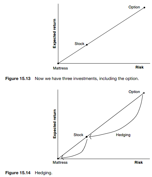
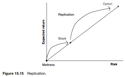
Option payoffs can be replicated by stocks and cash. So, we can get a risk-free investment using the option and the stock, and this is hedging. And, the stock can be replicated by cash and the option.
We say that markets are complete. The practical implication of complete markets is that options are hedgeable and therefore can be priced without any need to know probabilities.
The real and risk-neutral worlds
People often refer to the risk-neutral world in which people don’t care about risk. The risk-neutral world has the following characteristics:
- We don’t care about risk, and don’t expect any extra return for taking unnecessary risk
- We don’t ever need statistics for estimating probabilities of events happening
- We believe that everything is priced using simple expectations
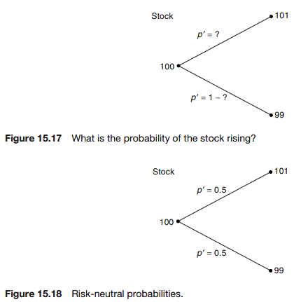
On the risk-neutral planet they calculate risk-neutral probabilities


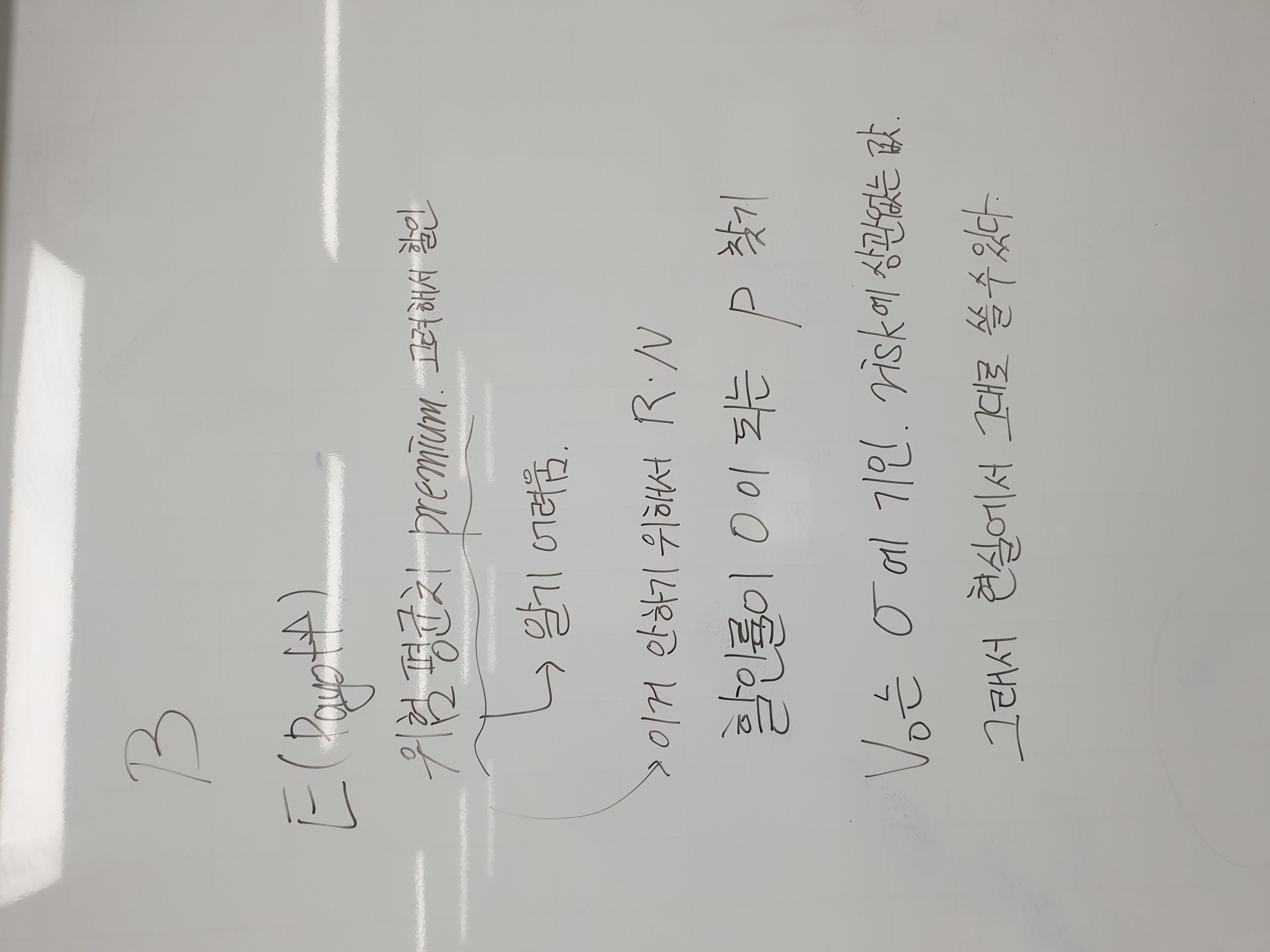
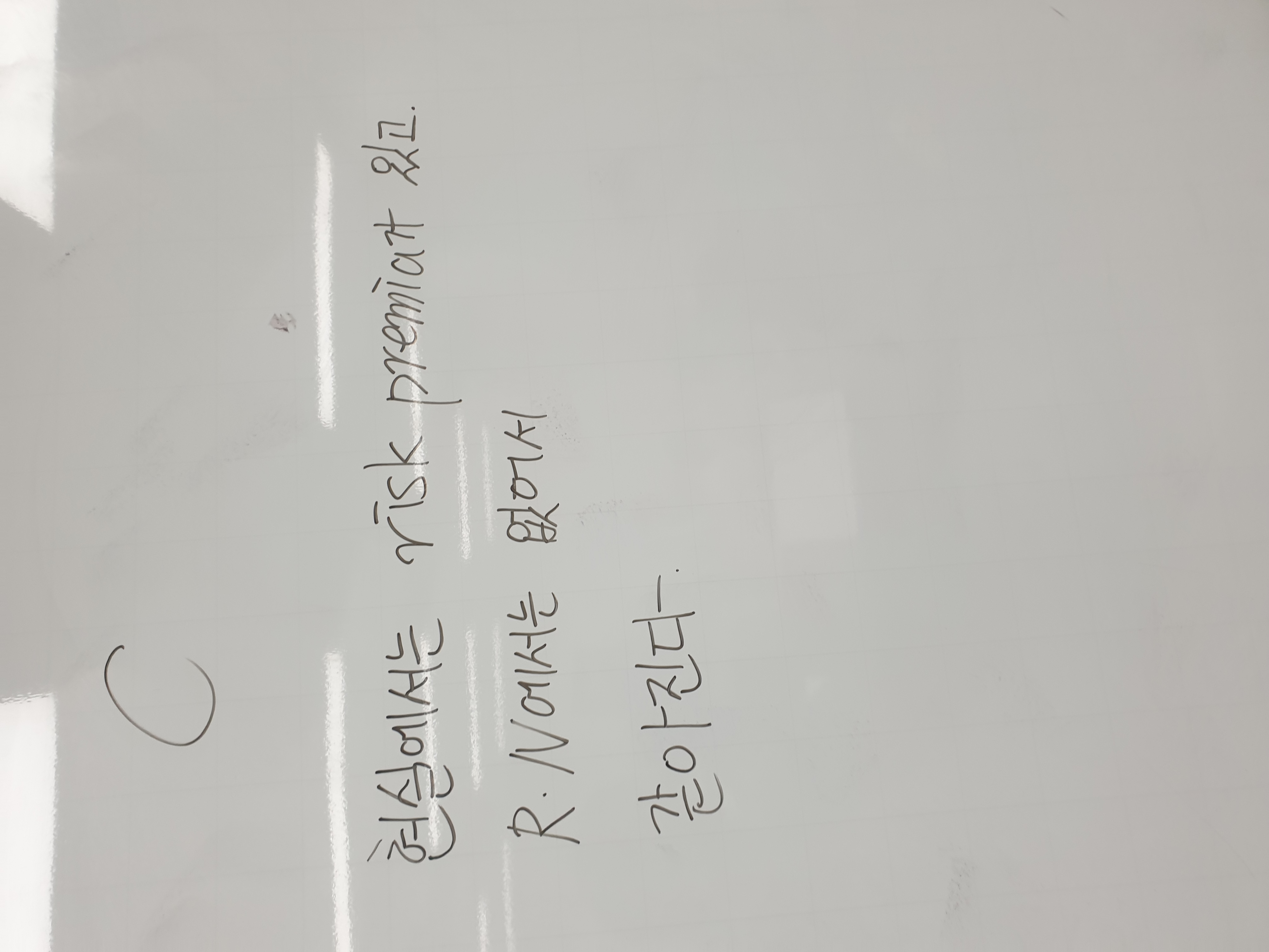
왜 option에서는 risk neutral pricing을 하는지, risk neutral pricing을 한 것을 현실에 사용해도 왜 괜찮은지
- 특히 왜 stock, bond에서는 risk averse로 이야기하다 derivatives 세계로 넘어오면 risk neutrality를 가정하는지
- risk neutral은 아주 특수한 상황인데, 왜 현실에서 가격을 계산한 것과 같은 결과를 벹어내는지
- 복제를 통해 옵션을 구현할 수 있으므로 가능한 일 - key idea
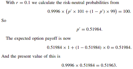
Non-zero interest rates
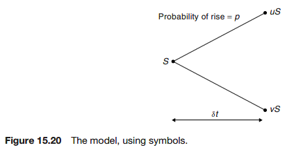
And now using symbols

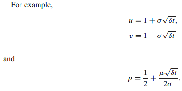
Average asset change

Standard deviation of asset price change
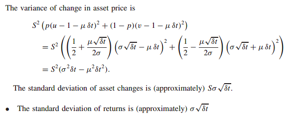
\(\delta t\)가 매우 작다고 가정하면, \(\delta t^2\)는 더 작기 때문에, approximately하게 \(\mu^2\delta t^2\)를 제거하고, variance of change in asset price를 \(S\sigma\sqrt{\delta t}\)라고 할 수 있다.
An equation for the value of an option
\[ \Pi = V - \Delta S \]
\[ V^+ - \Delta uS ~ or ~ V^- - \Delta vS \]
Hedging
\[ V^+ - \Delta uS = V^- - \Delta vS \]
\[ \Delta = \frac{V^+ - V^-}{(u - v)S} \]
\[ \Pi + \delta \Pi \]
This just means the original portfolio value plus the change in value.
In the risk-neutral world, there is the only one return, risk-free rate. Because whatever position investors take, the position can be hedged by derivatives with frictionless and no transaction costs.
No arbitrage
Since the value of the portfolio has been guaranteed, we can say that its value must coincide with the value of the original portfolio plus any interest earned at the risk-free rate; this is the no-arbitrage argument.
\[ \delta \Pi = r \Pi \delta t \]
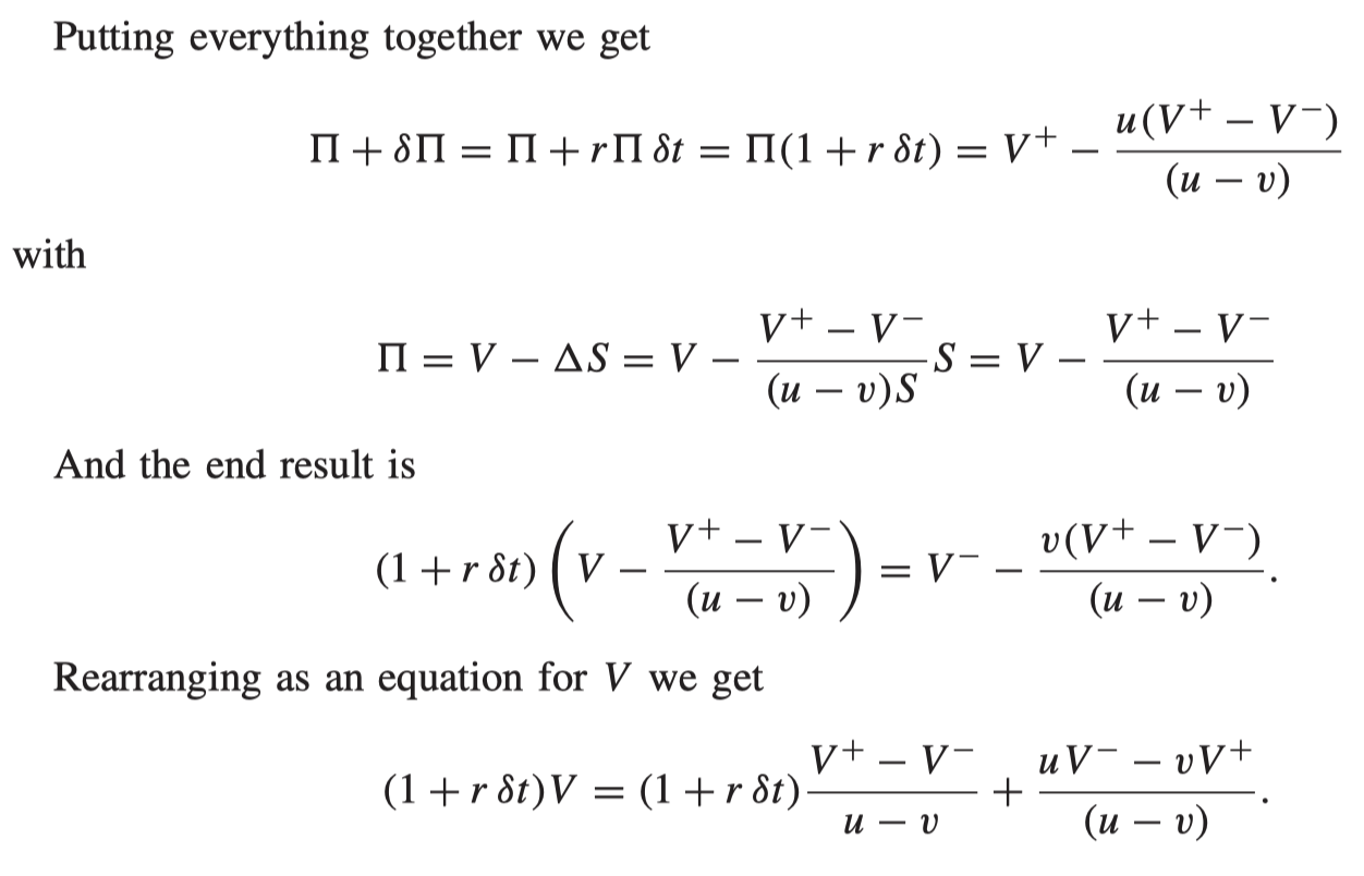

We could ‘say’ that the option price is the present value of an expectation. But not the real expectation.

The 2 expressions differ in the where one has the interest rate r the other has the drift \(\mu\), but otherwise they are the same.
- We call p’ the risk-neutral probability. It’s like the real probability, but the real probability if the drift rate were r instead of \(\mu\)
Where did the probability p go?
Interpreting p’ as a probability, the option value at any time is the present value of the risk-neutral expected value at any later time.
In readings, the expression ‘risk-neutral’ this or that, including the expression risk-neutral probability is not related to the real expectation.
Counterintuitive?

The binomial tree
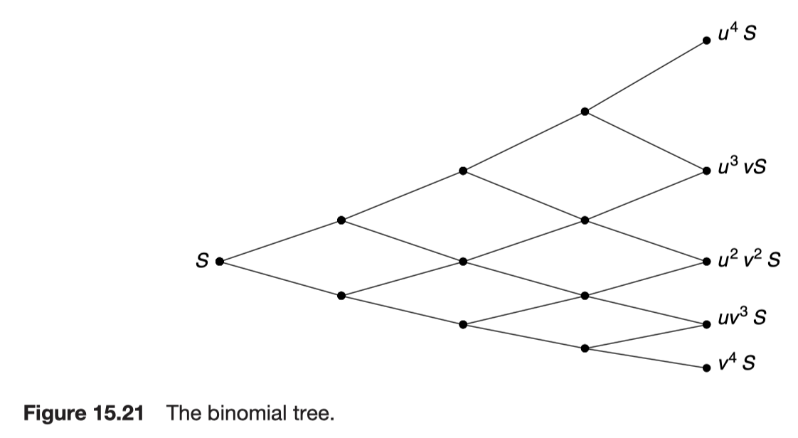
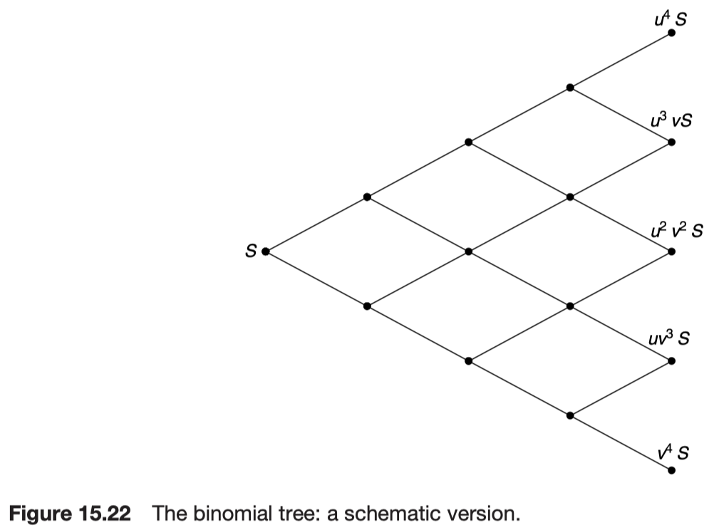
The binomial tree therefore contains within it an approximation to the probability density function for the lognormal random walk.
The asset price distribution
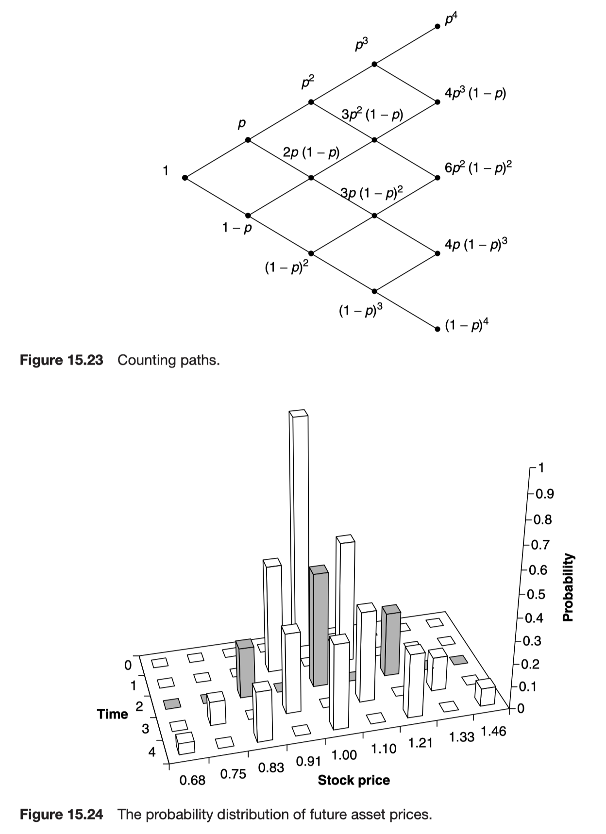
The probability of reaching a particular node in the binomial tree depends on the number of distinct paths to the node and the probabilities of the up and down moves. Since up and down moves are approximately equally likely and since there are more paths to the interior prices than to the 2 extremes, we will find that the probability distribution of future prices is roughly bell shaped.
Valuing back down the tree
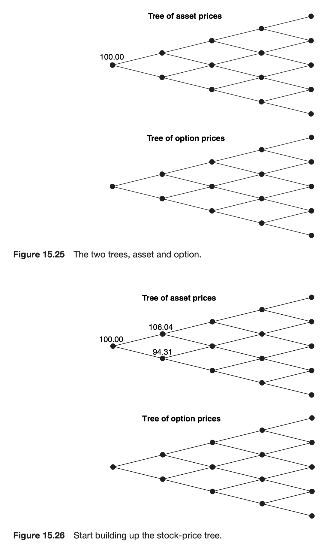
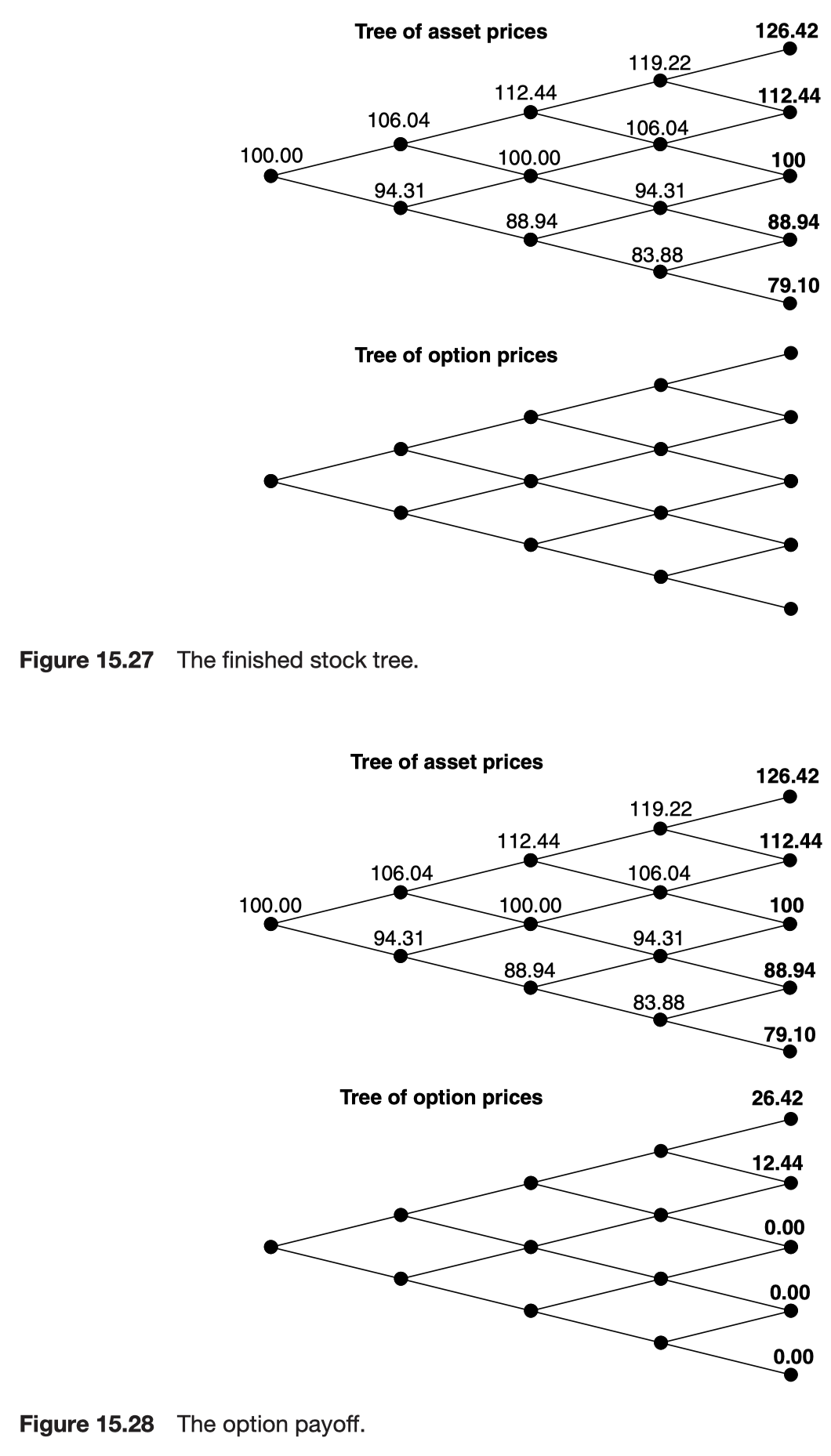
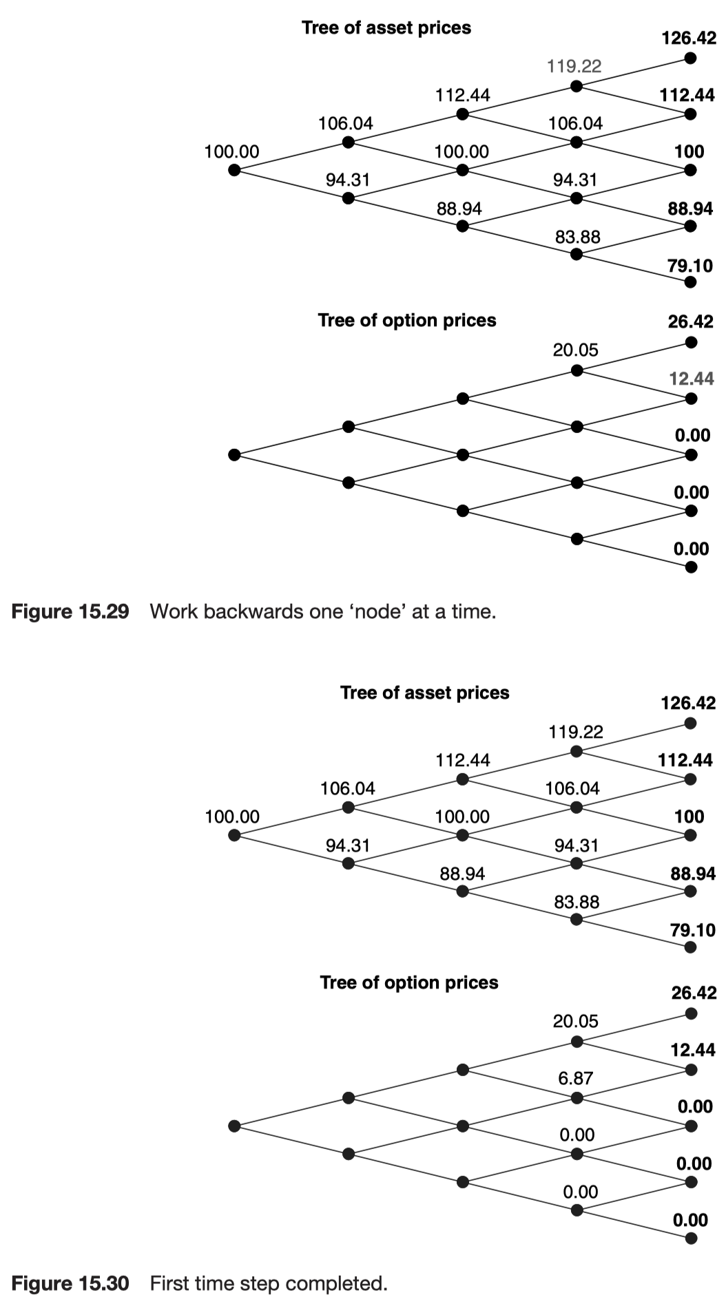
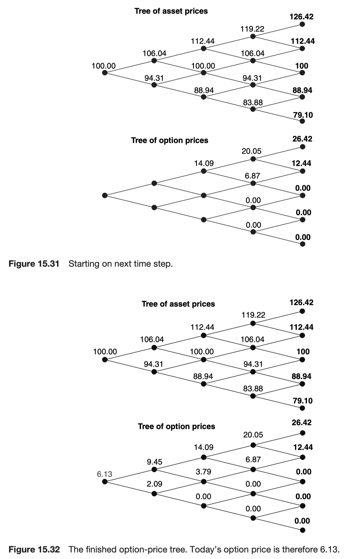
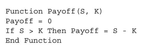
Programming the binomial method

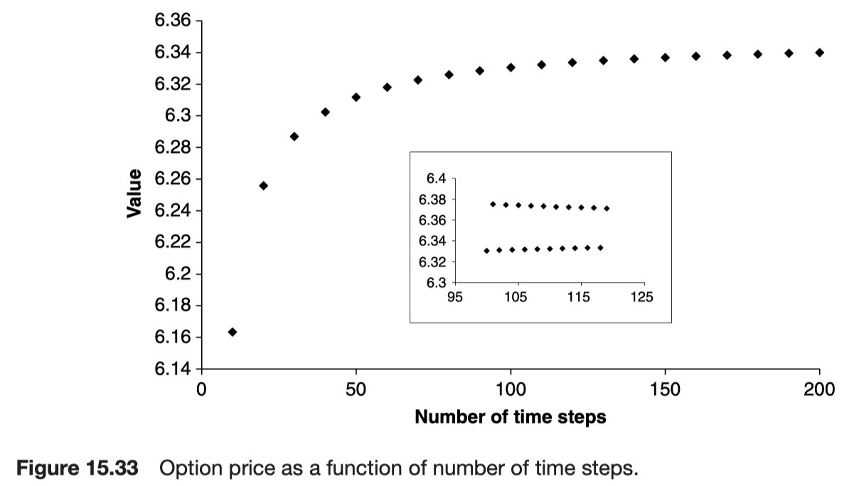
The odd number of time steps gives an answer that is too high and an even an answer that is too low.
The Greeks
From the binomial model the option’s delta is defined by
\[ \frac{V^+ - V^-}{(u - v)S} \]
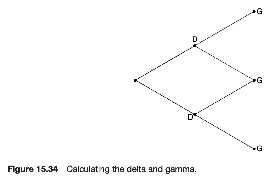
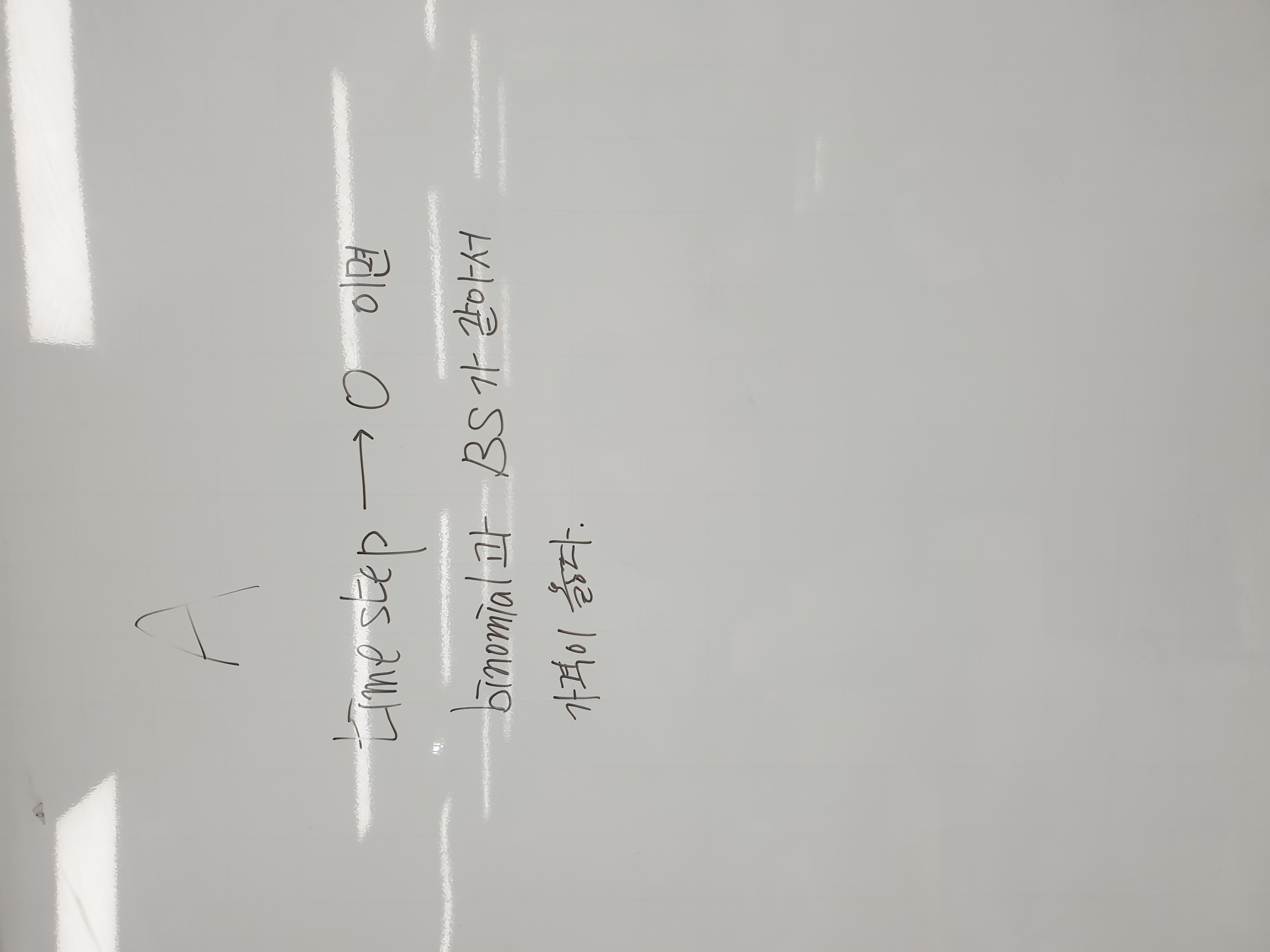
In the limit as the time step approaches zero, the delta becomes
\[ \frac{\partial V}{\partial S} \]
The gamma is
\[ \frac{\partial^2 V}{\partial S^2} \]
Gamma is a measure of how much we must rehedge at the next time step. The gamma is then the just the change in the delta from one of these to the other divided by the distance between them.
An obvious choice for the discrete-time definition of theta is to interpolate between V+ and V- to find a theoretical option value had *the asset not changed* and use this to estimate
\[ \frac{\partial V}{\partial t} \]
Why should not the asset changed for this estimation?
- Because theta of the binomial model has the Gamma term, for removing the gamma and representing the equation as a theta, this book assumes the asset should not change.
This results in
\[ \frac{\frac{1}{2}(V^+ + V^-) - V}{\delta t} \]
As the time step gets smaller and smaller these greeks approach the Black-Scholes continuous-time values.
The vega is
\[ \frac{\partial V}{\partial \sigma} \]
Using a binomial tree, there is two different values of \(\sigma\). Therefore, the vega is approximately by
\[ \frac{V^+ - V^-}{2\epsilon} \]
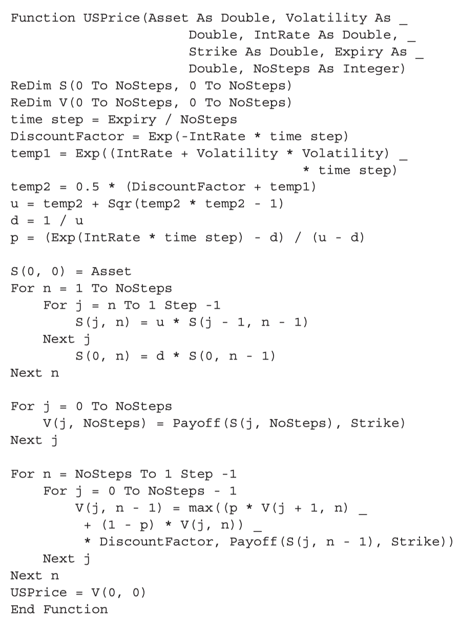
Early exercise


The continuous-time limit
Recalling that the Black-Sholes equation is in continuous time as \(\delta t \to 0\)
\[ u \sim 1 + \sigma \sqrt{\delta t} \]
\[ v \sim 1 - \sigma \sqrt{\delta t} \]
\[ V = V(S, t), ~ V^+ = V(uS, t + \delta t) ~ and ~ V^- = V(vS, t + \delta t) \]
\[ \Delta \sim \frac{\partial V}{\partial S} ~ as ~ \delta t \to 0 \]
\[ \frac{\partial V}{\partial t} + \frac{1}{2}\sigma^2 S^2 \frac{\partial^2 V}{\partial S^2} + rS \frac{\partial V}{\partial S} - rV = 0 \]
No arbitrage in the binomial, Black-Scholes and ‘other’ worlds
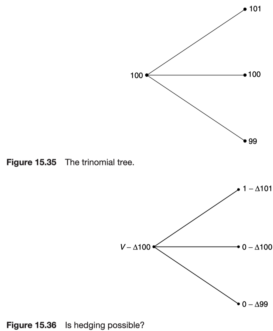
In the binomial discrete-time model and the Black-Scholes continuous-time model, it does not matter how the underlying asset moves, the resulting value of the portfolio is the same. For the trinomial random walk, we cannot choose a value for \(\Delta\) that ensures this to be the case. This amounts to solving 2 equations with just 1 unknown. Hedging is not possible in the trinomial world. Indeed, perfect hedging, and thus the application of the ‘no-arbitrage principle’ is only possible in the two special cases, the Black-Scholes continuous time/continuous asset world, and the binomial world. And in the far more complex ‘real’ world, delta hedging is not possible.
Further reading
