Quantitative Finance - Chapter 18 - portfolio management

Untitled.png

• Modern portfolio theory and the capital asset pricing model
• optimizing your portfolio
• alternative methodologies such as cointegration
• how to analyze portfolio performance

Introduction

The theory of derivatives pricing is theory of deterministic returns: we hedge our derivative with the underlying to eliminate risk, and our resulting risk-free portfolio then earns the risk-free rate of interest.

In this chapter, some of the theories behind the risk and reward of investment are introduced. Along the way, the benefits of diversification, how the return and risk on a portfolio of assets is related to the return and risk on the individual assets, and how to optimize a portfolio to get the best value for money.

For the most part, the assumptions are as follows

• We hold a portfolio for ‘a single period’ examining the behavior after this time
• During this period returns on assets are normally distributed
• The return on assets can be measured by an expected return (the drift) for each asset, a standard deviation of return (the volatility) for each asset and correlations between the asset returns.

Diversification

The portfolio value

$$\mathrm{\Pi }=\sum _{i=1}^N{w}_i{S}_i$$

At the end of the time horizon

$$\mathrm{\Pi }+\delta \mathrm{\Pi }=\sum _{i=1}^N{w}_i{S}_i(1+R_i)$$

The relative change in portfolio value

$$\frac{\delta \mathrm{\Pi }}{\mathrm{\Pi }}=\sum _{i=1}^N{W}_i{R}_i$$

$$W_i=\frac{w_i{S}_i}{\sum _{i=1}^N{w}_i{S}_i}$$

The expected return on the portfolio

$${\mu }_{\mathrm{\Pi }}=\frac{1}{T}E\left[\frac{\delta \mathrm{\Pi }}{\mathrm{\Pi }}\right]=\sum _{i=1}^N{W}_i{\mu }_i$$

the standard deviation of the return

$${\sigma }_{\mathrm{\Pi }}=\frac{1}{\sqrt{T}}\sqrt{var\left[\frac{\partial \mathrm{\Pi }}{\mathrm{\Pi }}\right]}=\sqrt{\sum _{i=1}^N\sum _{j=1}^N{W}_i{W}_j{\rho }_{ij}{\sigma }_i{\sigma }_j}$$

Uncorrelated assets

$${\mu }_{\mathrm{\Pi }}=\frac{1}{N}\sum _{i=1}^N{\mu }_i$$

$${\sigma }_{\mathrm{\Pi }}=\sqrt{\frac{1}{N^2}\sum _{i=1}^N{\sigma }_i^2}$$

• volatility or standard deviation as risk
• return as reward

Modern portfolio theory

Untitled

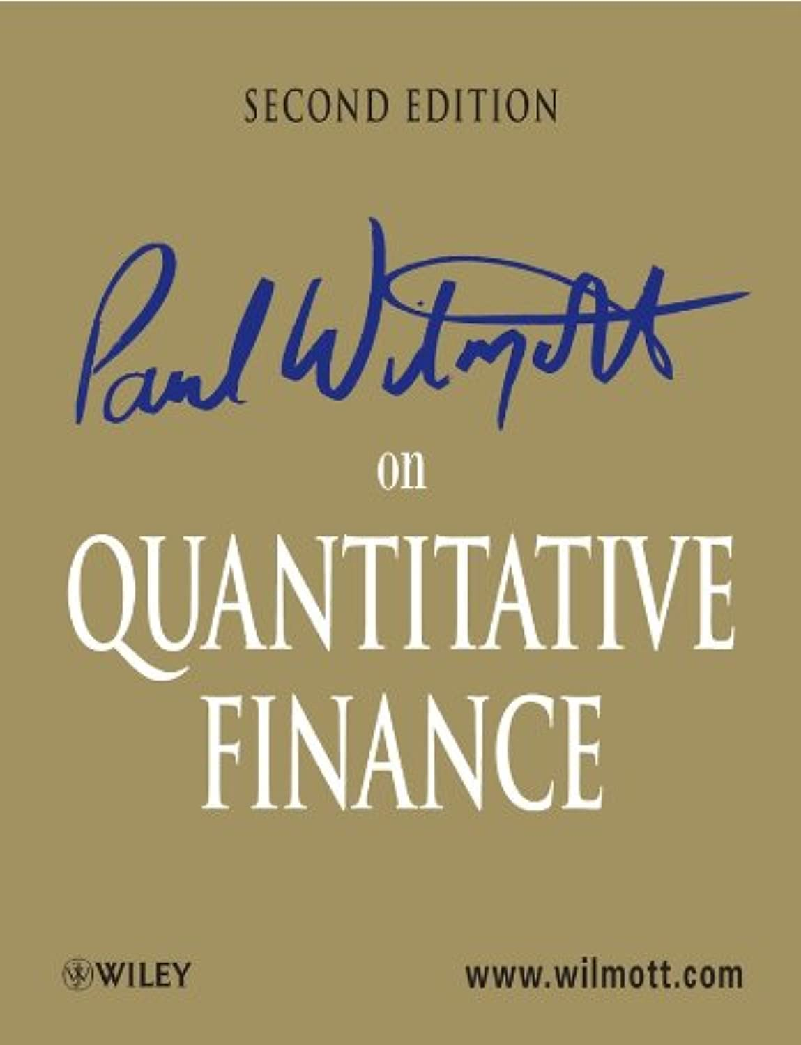
Harry Markowitz’s model provides a way of defining portfolios that are efficient. An efficient portfolio is one that has the highest reward for a given level of risk, or the lowest risk for a given reward.

A랑 E 사이가 아닌 밖으로 나가서 포지션을 잡으려면?

• 직선의 내분점/외분점을 생각해도 좋고
• A와 E 중에 어떤 자산을 short하고, 생긴 돈으로 추가적으로 long을 잡는다고 생각해도 좋음

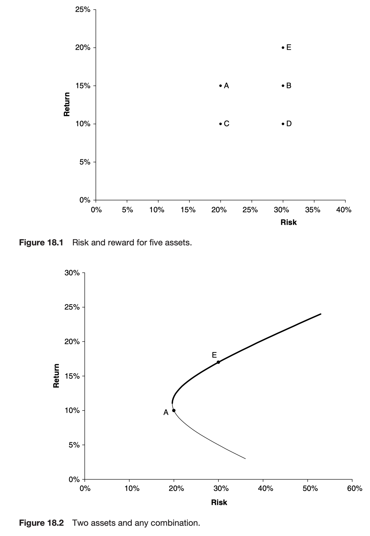
We cannot objectively say which out of A and E is the better; this is a subjective choice and depends on an investors’ risk preferences.

$${\mu }_{\mathrm{\Pi }}=W{\mu }_A+(1-W){\mu }_E$$

$${\sigma }_{\mathrm{\Pi }}^2=W^2{\sigma }_A^2+2W(1-W)\rho {\sigma }_A{\sigma }_E+(1-W{)}^2{\sigma }_E^2$$

mean의 W를 ${\mu }_{\mathrm{\Pi }}$에 대한 식으로 나타내서, variance 식의 W에 대입하면 쌍곡선 형태가 나타남

Untitled

When one of the volatilities is zero the line becomes straight. Anywhere on the curve between the two dots requires a long position in each asset. Outside this region, one of the assets is sold short to finance the purchase of the other.

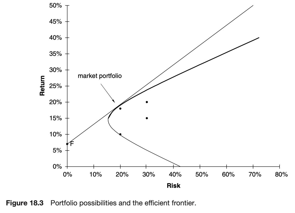
In this figure we can see the efficient frontier marked in bold. Given any choice of portfolio we would choose to hold one that lies on this efficient frontier.

Untitled

Including a risk-free investment

If we are allowed to hold this asset in our portfolio, then since the volatility of this asset is zero, we get the new efficient frontier which is the straight line in the figure. The portfolio for which the straight line touches the original efficient frontier is called the market portfolio. The straight line itself is called the capital market line.

Where do I want to be on the efficient frontier?

This is a personal choice, the efficient frontier is objective, given the data, but the ‘best’ position on it is subjective.

The return on portfolio $\mathrm{\Pi }$ is normally distributed because it is comprised of assets which are themselves normally distributed. It has mean ${\mu }_{\mathrm{\Pi }}$ and standard deviation ${\sigma }_{\mathrm{\Pi }}$.

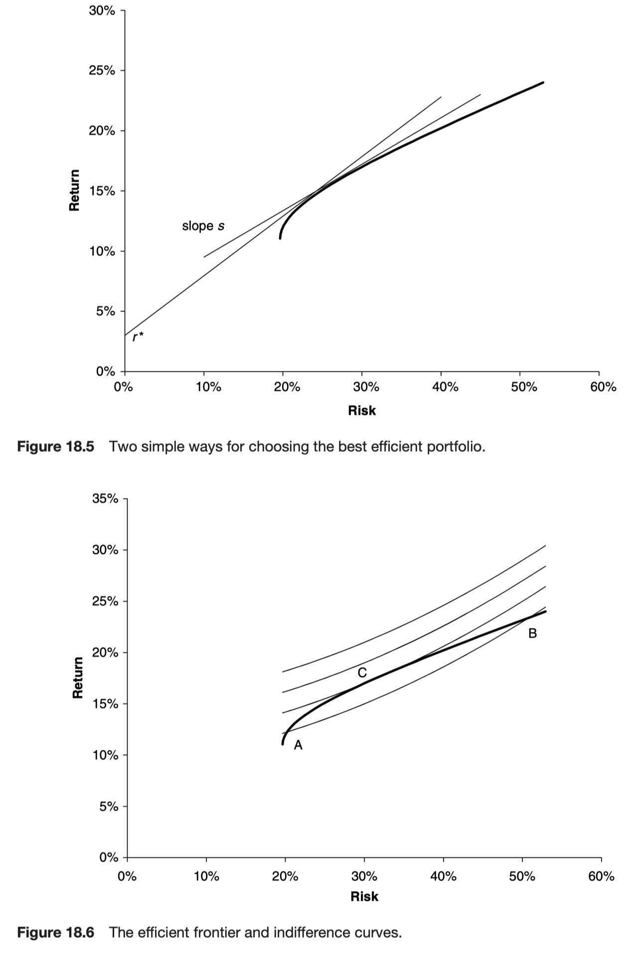
The slope of the line joining the portfolio $\mathrm{\Pi }$ to the risk-free asset is

$$s=\frac{{\mu }_{\mathrm{\Pi }}-r}{{\sigma }_{\mathrm{\Pi }}}$$

This is an important quantity; it is a measure of the likelihood of $\mathrm{\Pi }$ having a return that exceeds r. If C() is the cumulative distribution function for the standardized normal distribution then C(s) is the probability that the return on $\mathrm{\Pi }$ is at least r. More generally

$$C\left(\frac{{\mu }_{\mathrm{\Pi }}-r^{\ast }}{{\sigma }_{\mathrm{\Pi }}}\right)$$

is the probability that the return exceeds r. This suggests that if we want to minimize the chance of a return of less than r we should choose the portfolio from the efficient frontier set ${\mathrm{\Pi }}_{eff}$ with the largest value of the slope

$$\frac{{\mu }_{{\mathrm{\Pi }}_{eff}}-r^{\ast }}{{\sigma }_{{\mathrm{\Pi }}_{eff}}}$$

Conversely, if we keep the slope of this line fixed at s then we can say that with a confidence of C(s) we will lose no more than $${\mu }_{{\mathrm{\Pi }}_{eff}}-s{\sigma }_{{\mathrm{\Pi }}_{eff}}=r^{\ast }$$

Our portfolio choice could be determined by maximizing this quantity.

Neither of these methods give satisfactory results when there is a risk-free investment among the assets and there are unrestricted short sales, since they result in infinite borrowing.

• 왜 infinite borrowing이 일어나는지?
  • r를 maximize 해야 하는 상황인데, figure 18.5를 보면 r를 올리면 efficient frontier와 slope의 접점이 멀어지고, risk가 무한대로 가면서 infinite borrowing을 해야만 Sharpe Ratio를 극대화 할 수 있다.

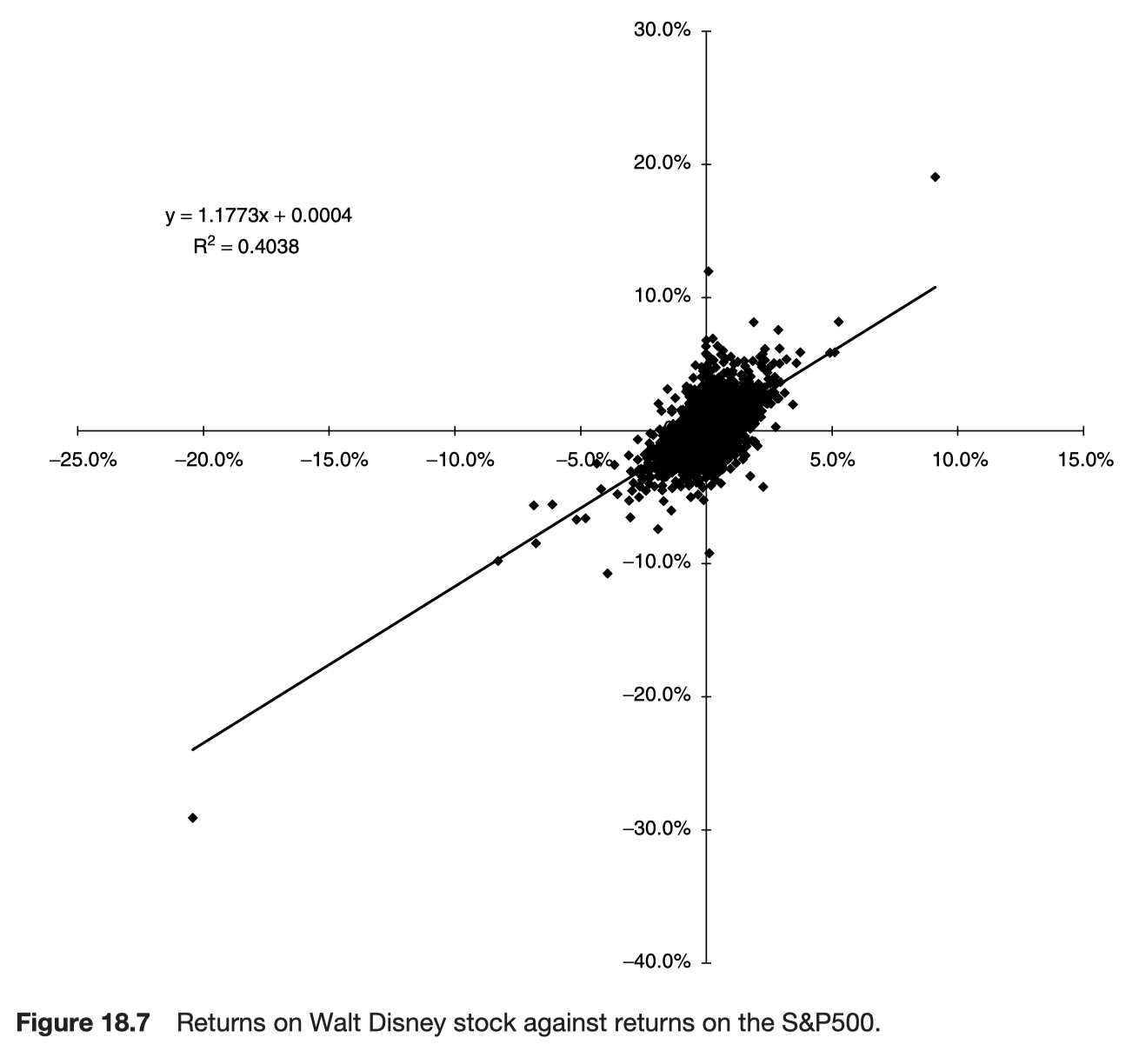
Another way of choosing the optimal portfolio is with the aid of a utility function. Indifference curves and the efficient frontier are called by this name because they are meant to represent lines along which the investor is indifferent to the risk/reward trade-off.

Untitled

• indifference curve는 어떻게 그려진 것인지?
  • risk averse한 경우에는 같은 추가위험에 더 많은 추가보상을 원하기 때문에 2차곡선/지수 형태로 급격하게 상승하는 형태를 가짐

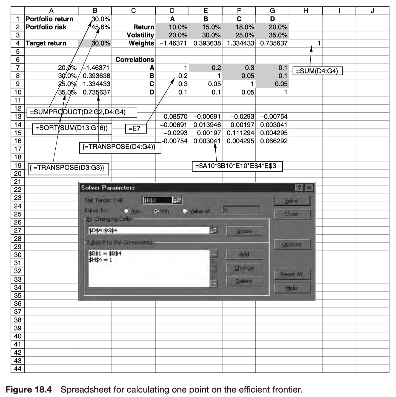
Markowitz in practice

The inputs to the Markowitz model are expected returns, volatilities and correlations. Most of these cannot be known accurately; only the volatilities are at all reliable.

Capital asset pricing model

The beta of an asset relative to a portfolio is the ratio of the covariance between the return on the security and the return on the portfolio to the variance of the portfolio.

$${\beta }_i=\frac{Cov[R_i{R}_M]}{Var[R_M]}$$

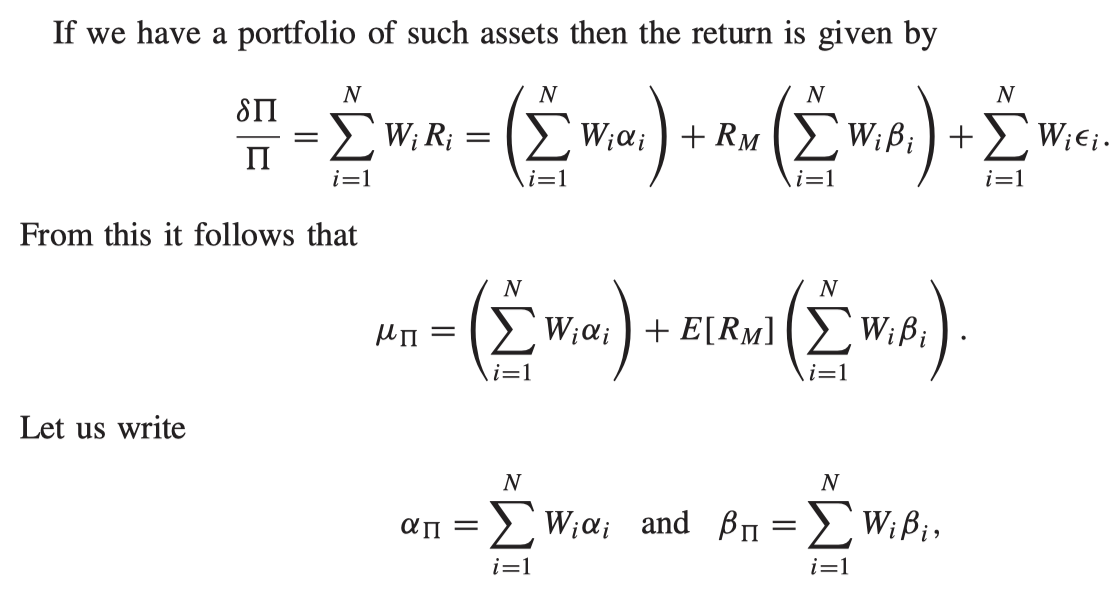
The single-index model

$$R_i={\alpha }_i+{\beta }_i{R}_M+{ϵ}_i$$

A constant drift, a random part common with the index M and a random part uncorrelated with the index ${ϵ}_i$. $\alpha$ and $\beta$ can be determined from a linear regression analysis.

$${\mu }_i={\alpha }_i+{\beta }_i{\mu }_M$$

$${\sigma }_i=\sqrt{{\beta }_i^2{\sigma }_M^2+e_i^2}$$

where $e_i$ is the standard deviation of ${ϵ}_i$

Untitled

Untitled

Untitled

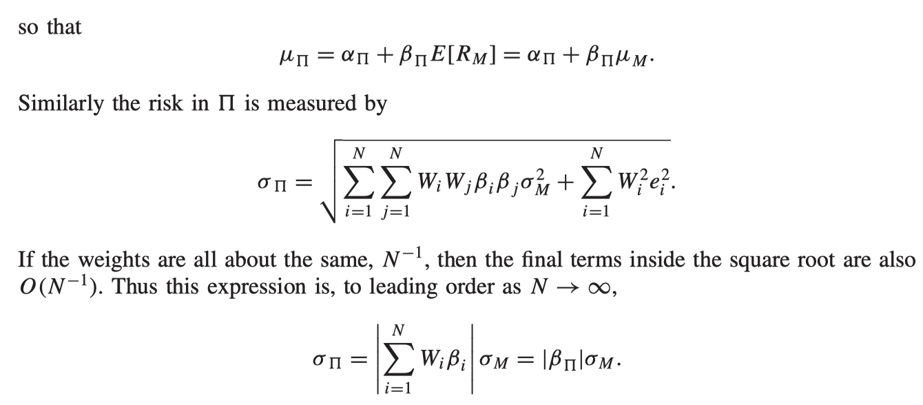
Observe that the contribution from the uncorrelated $ϵ$s to the portfolio vanishes as we increase the number of assets in the portfolio; The risk associated with the $ϵ$s is called diversifiable risk. The remaining risk, which is correlated with the index, is called systematic risk.

Choosing the optimal portfolio

The principal is the same as the Markowitz model for optimal portfolio choice. The only difference is that there are a low fewer parameters to be input, and the computation is a lot faster.

Choose a value for the portfolio return. Subject to this constraint, minimize ${\sigma }_{\mathrm{\Pi }}$. Repeat the minimization for different portfolio returns to obtain the efficient frontier. The position on this curve is then a subjective choice.

The multi-index model

$$R_i={\alpha }_i+\sum _{j=1}^n{\beta }_{ji}{R}_j+{ϵ}_i$$

Cointegration

Instead of asking whether 2 series are correlated we ask whether they are cointegrated.

To see whether 2 stocks stay close together we need a definition of stationary. A time series is stationary if it has finite and constant mean, standard deviation and autocorrelation function.

This is because the standard deviation of the sum grows like the square root of the number of throws. The mean may be zero but the sum is wandering further and further away from that mean.

• betting = adding up

Testing for the stationary of a time series $X_t$ involves a linear regression to find the coefficients, a, b and c in

$$X_t=a{X}_{t-1}+b+ct$$

• $|\alpha |>1$: the series is unstable → 발산
• $-1\le a<1$: the series is stationary
• a = 1: the series is non-stationary

As with all things statistical, we can only say that our value for a is accurate with a certain degree of confidence. To decide whether we have got a stationary or non-stationary series requires us to look at the Dickey-Fuller statistic to estimate the degree of confidence in our result. From this point on the subject of cointegration gets complicated.

Even though individual stock prices might be non-stationary it is possible for a linear combination to be stationary.

stationary를 판단하는 것이 degree of confidence의 문제이고, 이를 바탕으로 cointegration 여부를 판단하는데, finance에서는 일단 linear combination을 하고 stationary를 판단할 수 있으니 그냥 써도 된다 이런 말인가?

• regression으로는 a를 확신할 수 없으니, cointegration을 쓰는 것이 최신의 방법이다

https://en.wikipedia.org/wiki/Dickey–Fuller_test

In statistics, the Dickey–Fuller test tests the null hypothesis that a unit root is present in an autoregressive (AR) time series model. The alternative hypothesis is different depending on which version of the test is used, but is usually stationarity or trend-stationarity. The test is named after the statisticians David Dickey and Wayne Fuller, who developed it in 1979.

$$\sum _{i=1}^N{\lambda }_i=1,\sum _{i=1}^N{\lambda }_i{S}_i$$

If we can, then we say that stocks are cointegrated.

The important difference is that cointegration assumes far fewer properties for the individual time series. Most importantly, volatility and correlation do not appear explicitly.

Performance measurement

Common concept - return per unit risk

• Sharpe ratio: reward to variability
• Treynor ratio: reward to volatility

$$\text{Sharpe ratio}=\frac{{\mu }_{\mathrm{\Pi }}-r}{{\sigma }_{\mathrm{\Pi }}}$$

$$\text{Treynor ratio}=\frac{{\mu }_{\mathrm{\Pi }}-r}{{\beta }_{\mathrm{\Pi }}}$$

In these ${\mu }_{\mathrm{\Pi }}$ and ${\sigma }_{\mathrm{\Pi }}$ are the realized return and standard deviation for the portfolio over the period. The ${\beta }_{\mathrm{\Pi }}$ is a measure of the portfolio’s volatility.

Further reading

Untitled