- The relationship between option values and expectations for equities, currencies, commodities and indices
- the relationship between derivative products and expectations when interest rates are stochastic
- how to do Monte Carlo simulations to calculate derivative prices and to see the results of speculating with derivatives
- how to do simulations in many dimensions using Cholesky factorization
Relationship between derivative values and simulations: equities, indices, currencies, commodities
The fair value of an option in the Black-Scholes world is the present value of the expected payoff at expiry under a risk-neutral random walk for the underlying.
The risk-neutral random walk for S is
\[ dS = rS dt + \sigma S dX \]
\[ \text{option value} = e^{-r(T - t)}E[payoff(S)] \]
This result leads to an estimate for the value of an option by following these simple steps:
- Simulate the risk-neutral random walk, starting at today’s value of the asset \(S_0\), over the required time horizon. This time period starts today and continues until the expiry of the option. This gives one relization of the underlying price path.
- For this realization calculate the option payoff
- Perform many more such realizations over the time horizon
- Calculate the average payoff over all realizations
- Take the present value of this average, this is the option value
Generating paths
The initial part of this algorithm requires first of all the generation of random numbers from a standardized normal distribution.
\[ \delta S = r S \delta t + \sigma S \sqrt{\delta t} \phi \]
where \(\phi\) is drawn from a standardized normal distribution. This discrete way of simulating the time series for S is called the Euler method.
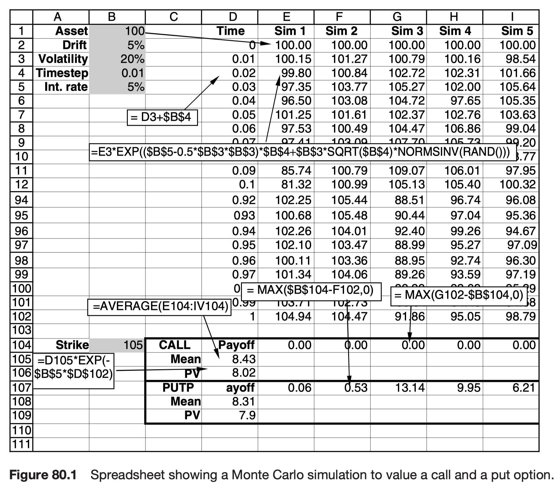
The method is particularly suitable for path-dependent options.
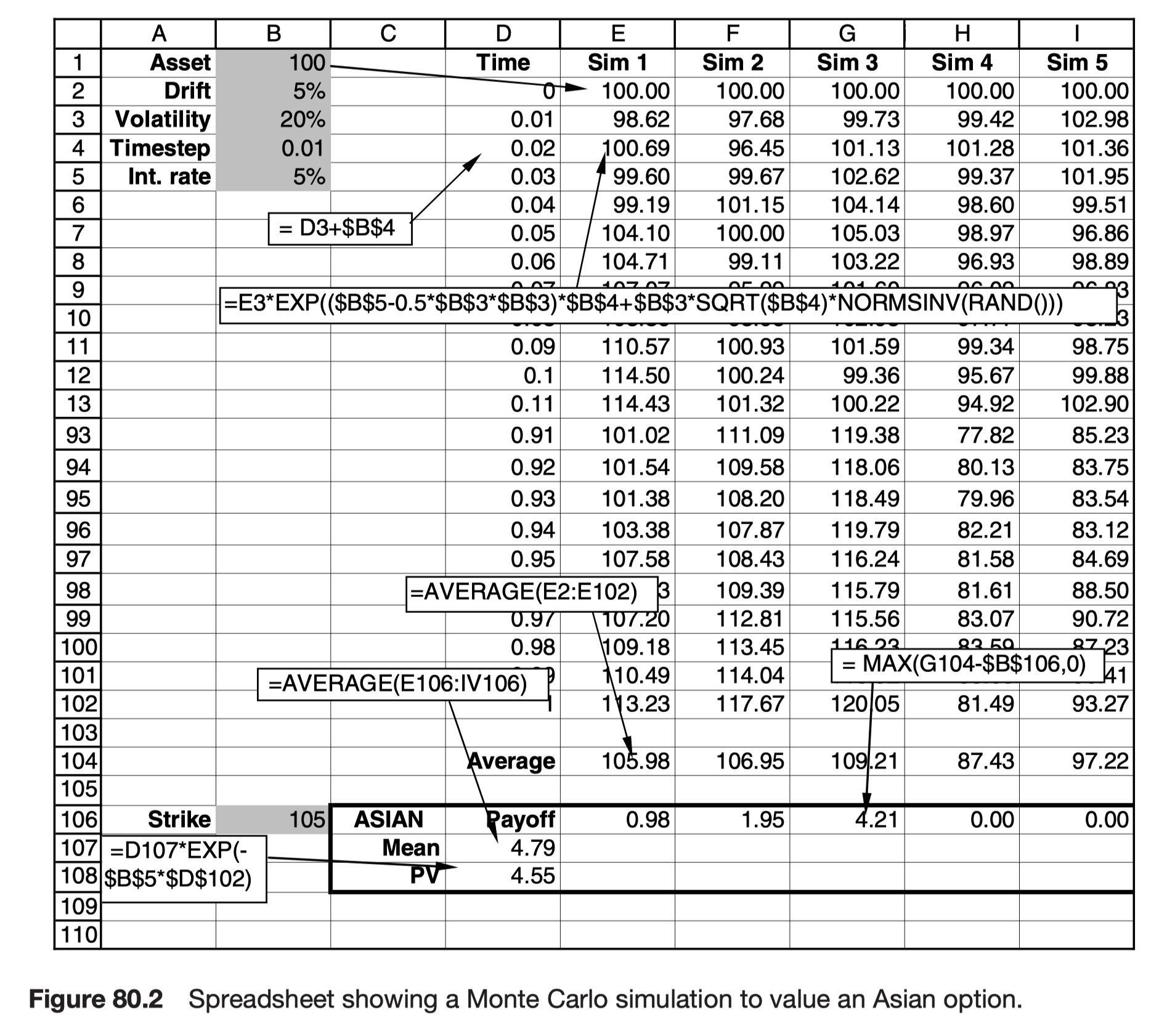
Lognormal underlying, no path dependency
\[ d(\log S) = (r - \frac{1}{2}\sigma^2)dt + \sigma dX \]
\[ S(t) = S(0) exp((r - \frac{1}{2}\sigma^2)t + \sigma \int_0^t{dX})) \]
\[ S(t + \delta t) = S(t) + \delta S = S(t) exp((r - \frac{1}{2}\sigma^2)\delta t + \sigma \sqrt{\delta t} \phi) \]
Advantages of Monte Carlo simulation
- The mathematics that you need to perform a Monte Carlo simulation can be very basic
- Correlations can be easily modeled
- There is plenty of software available, at the least there are spreadsheet functions that will suffice for most of the time
- To get a better accuracy, just run more simulations
- The effort in getting some answer is very low
- The models can often be changed without much work
- Complex path dependency can often be easily incorporated
- People accept the technique, and will believe your answers
Using random numbers
All we need are that the variance of the distribution must be finite and constant.
In the limit as the size of the time step goes to zero the simulations have the same probabilistic properties over a finite timescale regardless of the nature of the distribution over the infinitesimal timescale. This is a result of the central limit theorem.
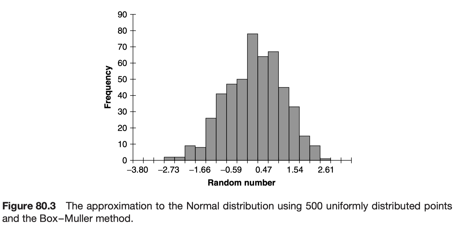
As I said above, it is best to use the exact expression (80.1) and then the choice of time step does not affect the accuracy of the random walk. In some cases we can take a single time step since the time stepping algorithm is exact. If we do use such a large time step then we must generate Normally distributed random variables. I will discuss this below, where I describe the Box–Muller method.
https://en.wikipedia.org/wiki/Box–Muller_transform
The Box–Muller transform, by George Edward Pelham Box and Mervin Edgar Muller, is a random number sampling method for generating pairs of independent, standard, normally distributed (zero expectation, unit variance) random numbers, given a source of uniformly distributed random numbers
If the size of the time step is δt then, for more complicated products, such as path-dependent ones, we may still introduce errors of O(δt) by virtue of the discrete approximation to continuous events
- finite number test를 infinite number of possible path로 하기 때문에 생기는 error인지?
\[ O(max(\delta t, \frac{1}{\sqrt{N}})) \]
To minimize this quantity, while keeping the total computing time fixed such that 3\(O(N / \delta t) = K\), we must choose
\[ N = O(K^{2/3}) ~ and ~ \delta t = O(K^{-1/3}) \]
Generating normal variables
To get a better approximation you can just add up more uniform random variables. The general formula is
\[ \sqrt{\frac{12}{N}}((\sum_{i = 1}^N{\psi_i}) - \frac{N}{2}) \]
Box-Muller
The Box–Muller method takes two uniform random numbers x1 and x2 between zero and one and combines them to give two numbers y1 and y2 that are both Normally distributed:
\[ y_1 = \sqrt{-2\ln x_1}cos(2\pi x_2) ~ and ~ y_2 = \sqrt{-2\ln x_1}sin(2\pi x_2) \]
Real versus risk neutral, speculation versus hedging
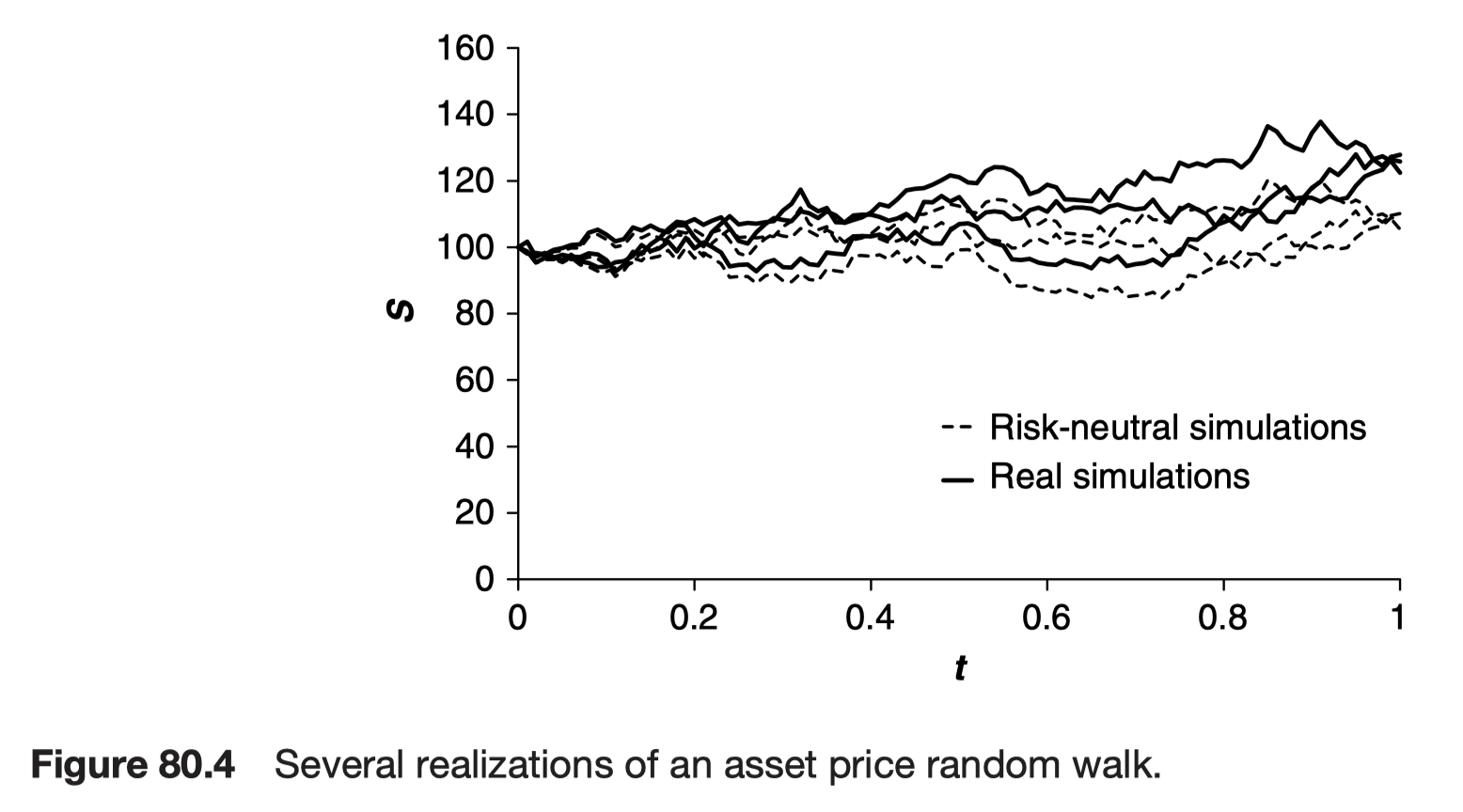
This is because in holding an unhedged position we cannot guarantee the return that we (theoretically) get from a hedged position. It is therefore valid and important to have the real drift as one of the parameters; it would be incorrect to estimate the probability density function for the return from an unhedged position using the risk-neutral drift.
Interest rate products
The correct way to estimate option value with stochastic interest rates is as follows:
- Simulate the random walk for the risk-adjusted spot interest rate r, as discussed below, starting at today’s value of the spot rate, over the required time horizon. This time period starts today and continues until the expiry of the option. This gives one realization of the spot rate path.
- For this realization calculate two quantities, the payoff and the average interest rate realized up until the payoff is received.
- Perform many more such realizations.
- For each realization of the r random walk calculate the present value of the payoff for this realization discounting at the average rate for this realization.
- Calculate the average present value of the payoffs over all realizations; this is the option value.

average interest rate으로 할인하는 이유는 risk-neutral world에서 모든 asset은 same risk-free growth rate을 가지기 때문


Calculating the Greeks

This is a central difference.
This is an accurate estimate of the first derivative, with an error of \(O(h^2)\). However, the error in the measurement of the two option values at S + h and S − h can be much larger than this for the Monte Carlo simulation. These Monte Carlo errors are then magnified when divided by h, resulting in an error of \(O(1/h N^{1/2})\). To overcome this problem, estimate the value of the option at S + h and S − h using the same values for the random numbers. In this way the errors in the Monte Carlo simulation will cancel each other out. The same principal is used to calculate the gamma and the theta of the option.
- 단일점에서 변화율인 delta를 구하면 역으로 오차가 커지니 central difference로 delta를 계산
- 이 마저도 error가 있음 - approximation이기 때문
The solution of the Black-Scholes partial differential equation
\[ \frac{\partial V}{\partial t} + \frac{1}{2}\sigma^2 S^2 \frac{\partial^2 V}{\partial S^2} + rS \frac{\partial V}{\partial S} - rV = 0 \]
has the interpretation of being the expected value of the present value of the payoff, under a risk-neutral random walk.
The first ‘r’ in this equation represents the ‘r’ in
\[ dS = rSdt + \sigma S dX \]
The second ‘r’ represents present valuing
\[ \frac{\partial \Delta}{\partial t} + \frac{1}{2}\sigma^2 S^2\frac{\partial^2 \Delta}{\partial S^2} + (r + \sigma^2)S\frac{\partial \Delta}{\partial S} = 0 \]
where
\[ \Delta = \frac{\partial V}{\partial S} \]


Higher dimensions: Cholesky factorization
Monte Carlo simulation is a natural method for the pricing of European-style contracts that depend on many underlying assets.

\(\phi_i\) are correlated
\[ E[\phi_i \phi_j] = \rho_{ij} \]
Cholesky factorization - generate correlated random variables
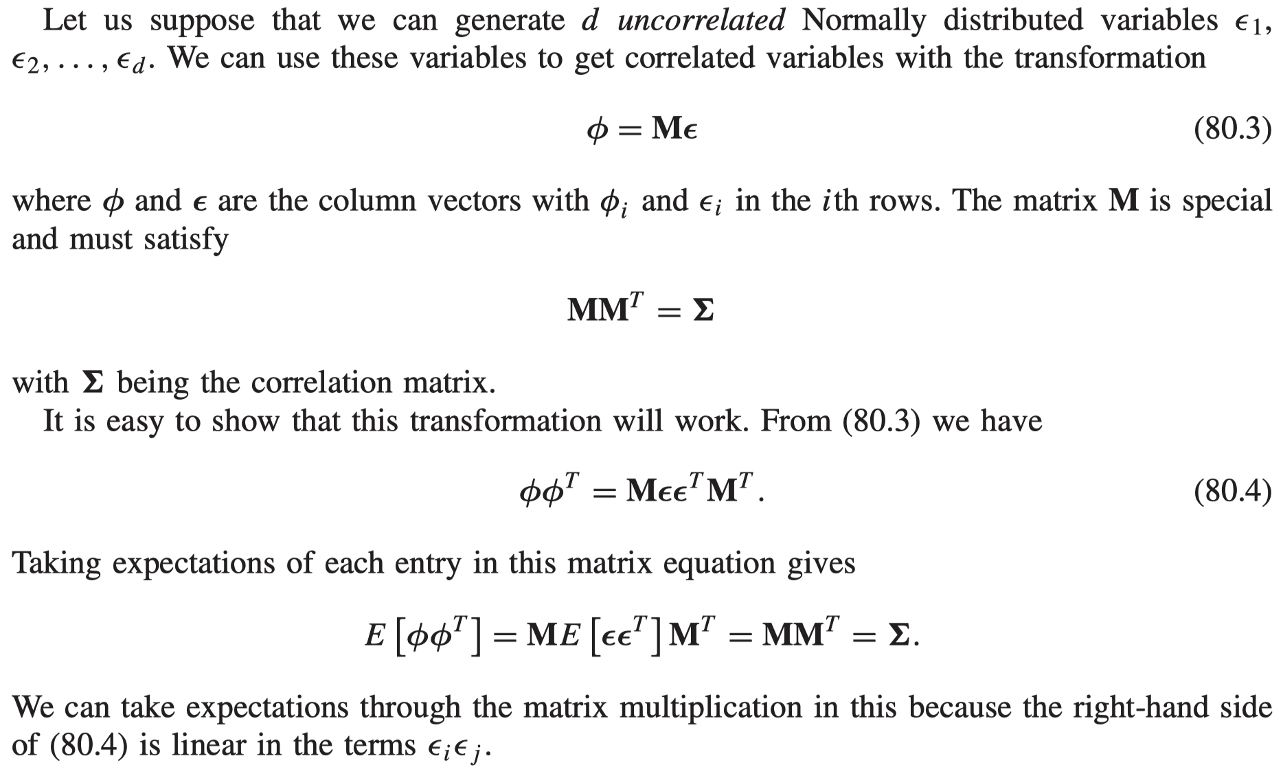
It results in a matrix M that is lower triangular.
Cholesky decomposition can become unstable if you have any perfect correlation.
Calculation time

Note that we don’t get the greeks from this calculation. If we want to calculate the greeks then we will have to repeat the calculation as many more times as we need greeks.
Speeding up convergence
Monte Carlo simulation is inefficient, compared with finite-difference methods, in dimensions less than about three.
Antithetic variables
- normal random number로 일단 asset price, option payoff, present value의 path를 구현
- sample을 추출하여 sign을 바꾸고
- 다시 simulation을 해서 option payoff, present value의 path를 구현
- 두 simulation의 평균을 구해서 option value로 사용
normal distribution의 symmetry 특성을 활용
Control variate technique
2개의 derivatives가 있다고 가정
- 하나는 우리가 value를 구하고 싶은 derivatives
- 다른 하나는 비슷한 structure를 가진 derivatives
하나의 realization으로 두 derivatives를 valuing하는 방법
simulation으로 구해진 value가 \(V_1', V_2'\)이고, 비슷한 derivatives의 실제 value가 \(V_2\)라면 첫 번째 derivatives의 value는
\[ V_1' - V_2' + V_2 \]
이렇게 표현하면 V1과 V2의 valuation에서의 error의 크기가 같다는 것을 가정하게 된다.
이 technique을 가다듬어서 만든 방법을 martingale variance reduction이라고 부른다.
- simulates one or more new dependent variables at the same time as the path of the underlying
- 각 시점에서 expected value가 0이 되도록 하는 stochastic variable을 선택
- 이 새로운 variable을 variate이라고 부름
- option 가격에 이 variate을 더해줌
Pros and cons of Monte Carlo simulations
장점
- exotic option, path-dependent derivatives의 가격을 쉽게 계산할 수 있음
단점
- solution이 있는 방법에 비해 너무 오래걸리고 느림
- American option을 제대로 simulation 할 수 없음
- American option은 optimal exercise point를 찾아야 하는데, 이는 t 시점부터 만기까지 모든 자산의 가격에 대해 계산해보아야 하는데
- Monte Carlo simulation은 단지 해당 시점의 option price만을 계산
- finite number of realization이라는 점에서 발생하는 error가 있음
- 이는 \(\epsilon / \sqrt{N}\)에 비례하는데, simulation 개수를 늘려서 error를 줄이는 방법이 있음
- 다만 이 역시 제일 처음 단점과 연결되어 시간이 오래 걸린다는 문제가 있음
American options
American option을 Monte Carlo simulation을 이용해 계산할 때 문제가 되는 부분은 바로 계산하는 time direction이다.
partial differential equation으로 계산할 경우 만기부터 현재까지 역산하여 value를 구하게 되는데, Monte Carlo simulation은 계산하는 현재 시점만을 기준으로 option의 가격을 구한다.
- 따라서 현 시점에 early-exercise를 판단할 수 없다
매 시점마다 asset price의 path를 그려서 early exercise 여부를 판단할 수는 있겠지만 이는 computationally time-consuming한 작업이다.
Longstaff & Schwartz regression approach for American options
Monte Carlo simulation으로 American option을 valuation하는 방법에는 Longstaff & Schwartz가 2001년 발표한 알고리즘이 가장 유명하다.
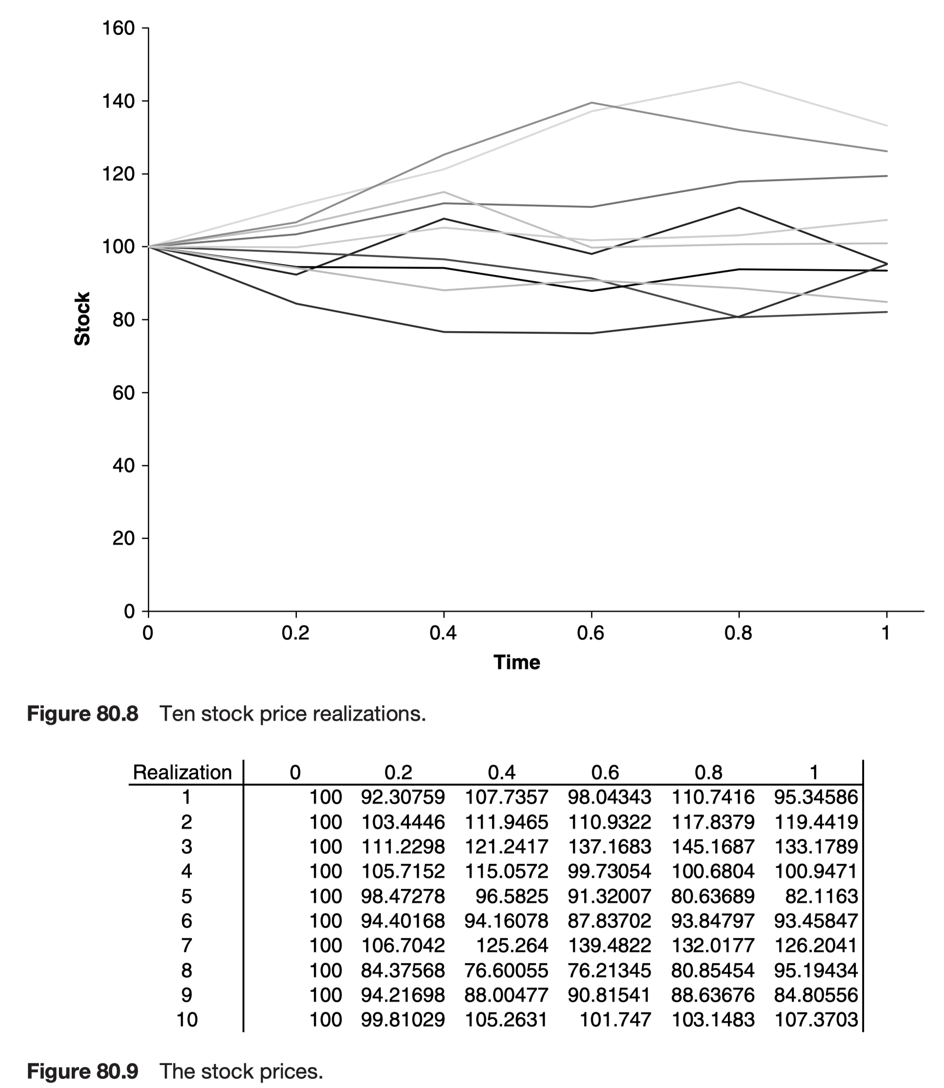
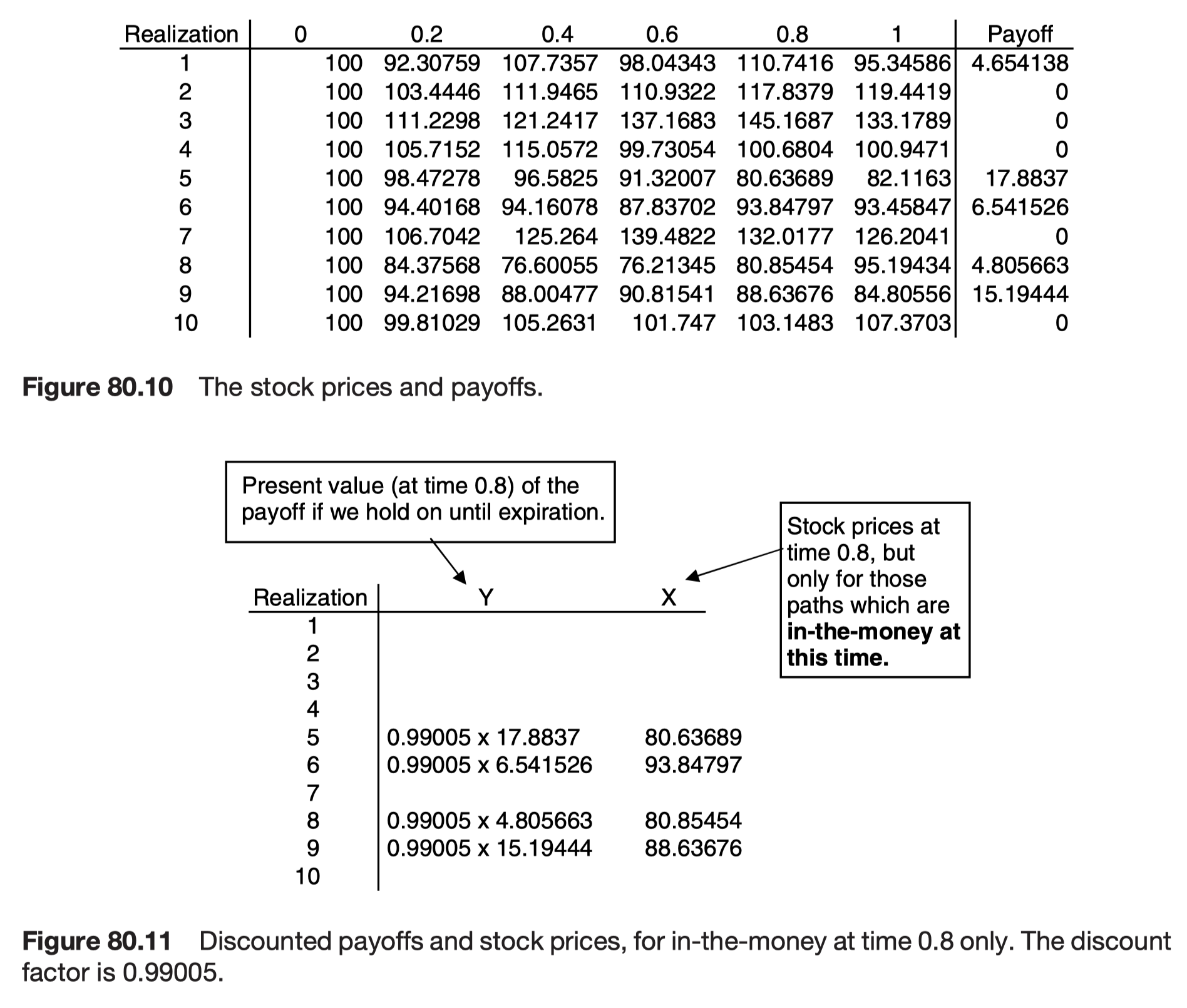
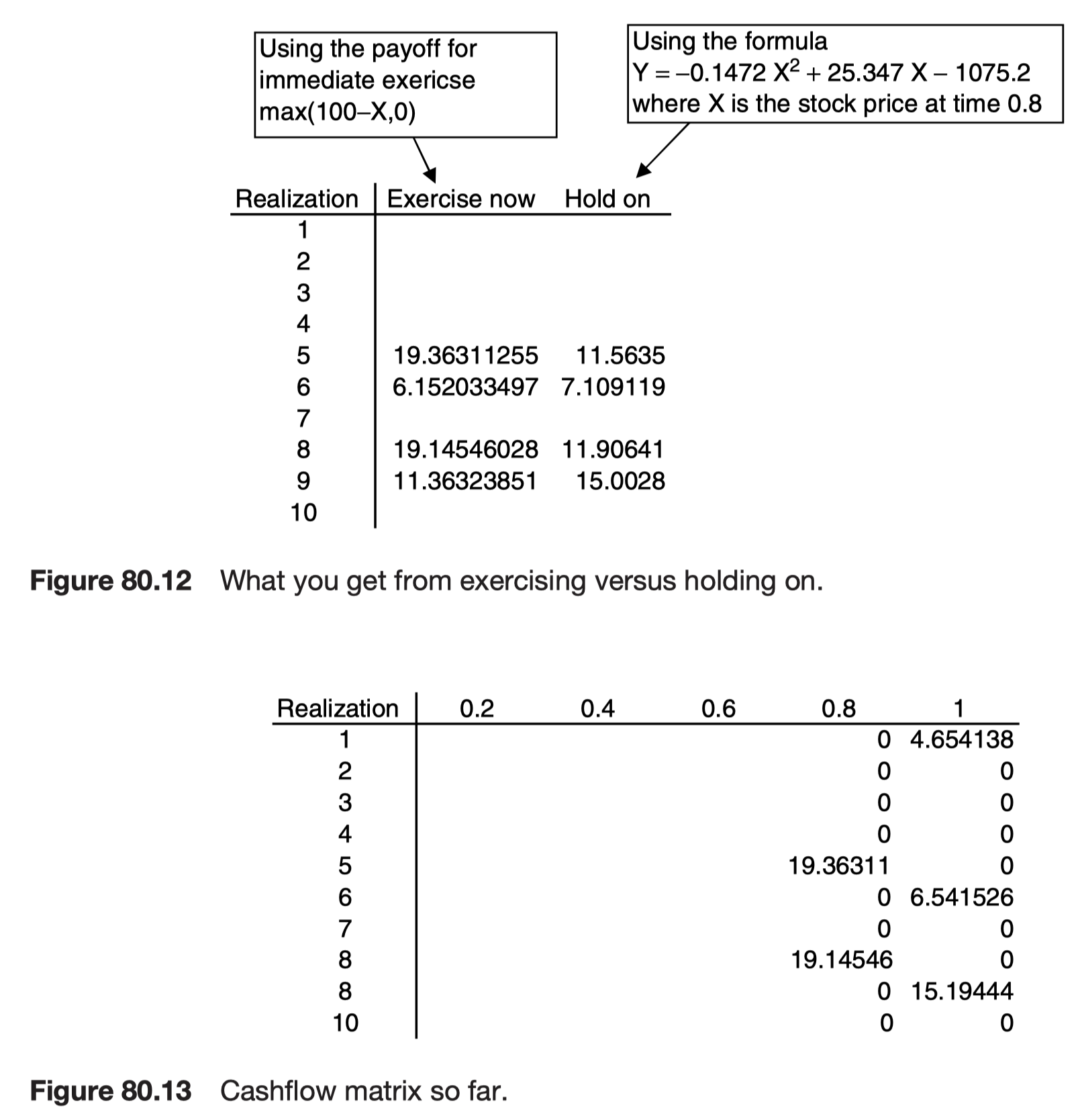
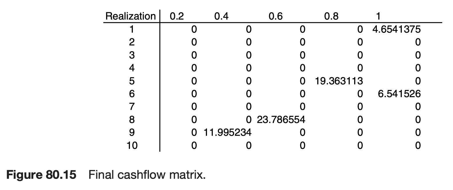
forward simulation은 그대로 하고, 각 시점마다 cashflow의 현재가치를 계산하지만, 각 단계마다 단순회귀를 사용하여 early exercise 여부를 판단한다.

Further reading

